Goodness of fit tests for continuous time financial market models
Bạn đang xem bản rút gọn của tài liệu. Xem và tải ngay bản đầy đủ của tài liệu tại đây (1.89 MB, 99 trang )
GOODNESS-OF-FIT TESTS FOR CONTINUOUS-TIME
FINANCIAL MARKET MODELS
YANG LONGHUI
NATIONAL UNIVERSITY OF SINGAPORE
2004
GOODNESS-OF-FIT TESTS FOR CONTINUOUS-TIME
FINANCIAL MARKET MODELS
YANG LONGHUI
(B.Sc. EAST CHINA NORMAL UNIVERSITY)
A THESIS SUBMITTED
FOR THE DEGREE OF MASTER OF SCIENCE
DEPARTMENT OF STATISTICS AND APPLIED PROBABILITY
NATIONAL UNIVERSITY OF SINGAPORE
2004
i
Acknowledgements
I would like to extend my eternal gratitude to my supervisor, Assoc. Prof.
Chen SongXi, for all his invaluable suggestions and guidance, endless patience and
encouragement during the mentor period. Without his patience, knowledge and
support throughout my studies, this thesis would not have been possible.
This thesis, I would like to contribute to my dearest family who have always
been supporting me with their encouragement and understanding in all my years.
To He Huiming, my husband, thank you for always standing by me when the nights
were very late and the stress level was high. I am forever grateful for your sacrificing
your original easy life for companying with me in Singapore.
Special thanks to all my friends who helped me in one way or another for their
friendship and encouragement throughout the two years. And finally, thanks are
due to everyone at the department for making everyday life enjoyable.
ii
Contents
1 Introduction
1
1.1
A Brief Introduction To Diffusion Processes . . . . . . . . . . . . .
1
1.2
Notation . . . . . . . . . . . . . . . . . . . . . . . . . . . . . . . . .
3
1.3
Commonly Used Diffusion Models . . . . . . . . . . . . . . . . . . .
4
1.4
Parameter Estimation . . . . . . . . . . . . . . . . . . . . . . . . .
7
1.5
Nonparametric Estimation . . . . . . . . . . . . . . . . . . . . . . .
10
1.6
Methodology And Main Results . . . . . . . . . . . . . . . . . . . .
13
1.7
Chapter Development . . . . . . . . . . . . . . . . . . . . . . . . . .
14
2 Existing Tests For Diffusion Models
16
2.1
Introduction . . . . . . . . . . . . . . . . . . . . . . . . . . . . . . .
16
2.2
A¨ıt-Sahalia’s Test . . . . . . . . . . . . . . . . . . . . . . . . . . . .
18
2.2.1
Test Statistic . . . . . . . . . . . . . . . . . . . . . . . . . .
18
2.2.2
Distribution Of The Test Statistic . . . . . . . . . . . . . .
20
Pritsker’s Study . . . . . . . . . . . . . . . . . . . . . . . . . . . . .
21
2.3
ii
CONTENTS
iii
3 Goodness-of-fit Test
26
3.1
Introduction . . . . . . . . . . . . . . . . . . . . . . . . . . . . . . .
26
3.2
Empirical Likelihood . . . . . . . . . . . . . . . . . . . . . . . . . .
28
3.2.1
The Full Empirical Likelihood . . . . . . . . . . . . . . . . .
28
3.2.2
The Least Squares Empirical Likelihood . . . . . . . . . . .
34
Goodness-of-fit Test . . . . . . . . . . . . . . . . . . . . . . . . . . .
37
3.3
4 Simulation Studies
41
4.1
Introduction . . . . . . . . . . . . . . . . . . . . . . . . . . . . . . .
41
4.2
Simulation Procedure . . . . . . . . . . . . . . . . . . . . . . . . . .
42
4.3
Simulation Result . . . . . . . . . . . . . . . . . . . . . . . . . . . .
46
4.3.1
Simulation Result For IID Case . . . . . . . . . . . . . . . .
46
4.3.2
Simulation Result For Diffusion Processes . . . . . . . . . .
50
Comparing With Early Study . . . . . . . . . . . . . . . . . . . . .
63
4.4.1
Pritsker’s Studies . . . . . . . . . . . . . . . . . . . . . . . .
63
4.4.2
Simulation On A¨ıt-Sahalia(1996a)’s Test . . . . . . . . . . .
63
4.4
5 Case Study
66
5.1
The Data . . . . . . . . . . . . . . . . . . . . . . . . . . . . . . . .
66
5.2
Early Study . . . . . . . . . . . . . . . . . . . . . . . . . . . . . . .
68
5.3
Test . . . . . . . . . . . . . . . . . . . . . . . . . . . . . . . . . . .
77
CONTENTS
iv
Summary
Diffusion processes have wide applications in many disciplines, especially in
modern finance. Due to their wide applications, the correctness of various diffusion
models needs to be verified. This thesis concerns the specification test of diffusion models proposed by A¨ıt-Sahalia (1996a). A serious doubt on A¨ıt-Sahalia’s
test in general and the employment of the kernel method in particular has been
cast by Pritsker (1998) by carrying out some simulation studies on the empirical
performance of A¨ıt-Sahalia’s test. He found that A¨ıt-Sahalia’s test had very poor
empirical size relative to nominal size of the test. However, we found that the
dramatic size distortion is due to the use of the asymptotic normality of the test
statistic. In this thesis, we reformulate the test statistic of A¨ıt-Sahalia by a version
of the empirical likelihood. To speed up the convergence, the bootstrap is employed
to find the critical values of the test statistic. The simulation results show that the
proposed test has reasonable size and power, which then indicate there is nothing
wrong with using the kernel method in the test of specification of diffusion models.
The key is how to use it.
v
List of Tables
1.1
Alternative specifications of the spot interest rate process . . . . . .
5
2.1
Common used Kernels (I(·) signifies the indicator function) . . . . .
20
2.2
Models considered by Pritsker (1998) . . . . . . . . . . . . . . . . .
23
2.3
Empirical rejection frequencies using asymptotic critical values at
5% level, extracted from Pritsker(1998). . . . . . . . . . . . . . . .
25
4.1
Optimal bandwidth corresponding different sample size . . . . . . .
45
4.2
Size of the bootstrap based LSEL Test for IID for a set of bandwidth
values and their sample sizes of 100, 200 and 500 . . . . . . . . . .
48
Size of the bootstrap based LSEL Test for the Vasicek model -2 for a
set of bandwidth values and their sample sizes of 120, 250, 500 and
1000 . . . . . . . . . . . . . . . . . . . . . . . . . . . . . . . . . . .
51
Size of the bootstrap based LSEL Test for the Vasicek model -1 for a
set of bandwidth values and their sample sizes of 120, 250, 500 and
1000 . . . . . . . . . . . . . . . . . . . . . . . . . . . . . . . . . . .
52
Size of the bootstrap based LSEL Test for the Vasicek model 0 for a
set of bandwidth values and their sample sizes of 120, 250, 500 and
1000 . . . . . . . . . . . . . . . . . . . . . . . . . . . . . . . . . . .
53
4.3
4.4
4.5
v
LIST OF TABLES
4.6
4.7
4.8
4.9
5.1
5.2
5.3
vi
Size of the bootstrap based LSEL Test for the Vasicek model 1 for
a set of bandwidth values and their sample sizes of 120, 250, 500,
1000 and 2000 . . . . . . . . . . . . . . . . . . . . . . . . . . . . . .
54
Size of the bootstrap based LSEL Test for the Vasicek model 2 for
a set of bandwidth values and their sample sizes of 120, 250, 500,
1000 and 2000 . . . . . . . . . . . . . . . . . . . . . . . . . . . . . .
55
Power of the bootstrap based LSEL Test for the CIR model for a
set of bandwidth values and their sample sizes of 120, 250, 500 . . .
62
Empirical rejection frequencies using asymptotic critical values at
5% level from Normal distribution. . . . . . . . . . . . . . . . . . .
64
Test statistics and P-values (P-V1 ) of Vasicek Model and CIR Model
of the empirical tests for the marginal density for the Fed fund rate
data, and P-values (P-V2 ) when the asymptotic normal distribution
is applied and the corresponding standard test statistics show in
brackets. . . . . . . . . . . . . . . . . . . . . . . . . . . . . . . . .
80
Test statistics and P-values (P-V1 ) of Inverse CIR Model and CEV
Model of the empirical tests for the marginal density for the Fed
fund rate data, and P-values (P-V2 ) when the asymptotic normal
distribution is applied and the corresponding standard test statistics
show in brackets. . . . . . . . . . . . . . . . . . . . . . . . . . . . .
81
Test statistics and P-values (P-V1 ) of Nonlinear Drift Model of
the empirical tests for the marginal density for the Fed fund rate
data, and P-values (P-V2 ) when the asymptotic normal distribution
is applied and the corresponding standard test statistics show in
brackets. . . . . . . . . . . . . . . . . . . . . . . . . . . . . . . . .
82
vii
List of Figures
4.1
4.2
4.3
4.4
4.5
4.6
4.7
Graphical illustrations of Table 4.2, where h* are the optimal bandwidths given in Table 4.1 and are indicated by vertical lines. . . . .
49
Graphical illustrations of Table 4.3 for the Vasicek model -2, where
h* are the optimal bandwidth given in Table 4.1 and are indicated
by the vertical lines. . . . . . . . . . . . . . . . . . . . . . . . . . .
56
Graphical illustrations of Table 4.4 for the Vasicek model -1, where
h* are the optimal bandwidth given in Table 4.1 and are indicated
by the vertical lines. . . . . . . . . . . . . . . . . . . . . . . . . . .
57
Graphical illustrations of Table 4.5 for the Vasicek model 0, where
h* are the optimal bandwidth given in Table 4.1 and are indicated
by the vertical lines. . . . . . . . . . . . . . . . . . . . . . . . . . .
58
Graphical illustrations of Table 4.6 for the Vasicek model 1, where
h* are the optimal bandwidth given in Table 4.1 and are indicated
by the vertical lines. . . . . . . . . . . . . . . . . . . . . . . . . . .
59
Graphical illustrations of Table 4.7 for the Vasicek model 2, where
h* are the optimal bandwidth given in Table 4.1 and are indicated
by the vertical lines. . . . . . . . . . . . . . . . . . . . . . . . . . .
60
Size of A¨ıt-Sahalia(1996a) Test for the Vasicek models for a set of
bandwidth values and their sample sizes of 120, 250, 500 . . . . . .
65
vii
LIST OF FIGURES
5.1
5.2
5.3
5.4
5.5
5.6
viii
The Federal Fund Rate Series between January 1963 and December
1998. . . . . . . . . . . . . . . . . . . . . . . . . . . . . . . . . . .
67
Nonparametric kernel estimates, parametric and smoothed parametric estimates of the marginal density for the Federal Fund Rate Data
and R1=0.031, R2=0.138. . . . . . . . . . . . . . . . . . . . . . . .
72
Nonparametric kernel estimates, parametric and smoothed parametric estimates of the marginal density for the Federal Fund Rate Data
and R1=0.031, R2=0.138. . . . . . . . . . . . . . . . . . . . . . . .
73
Nonparametric kernel estimates, parametric and smoothed parametric estimates of the marginal density for the Federal Fund Rate Data
and R1=0.031, R2=0.138. . . . . . . . . . . . . . . . . . . . . . . .
74
Nonparametric kernel estimates, parametric and smoothed parametric estimates of the marginal density for the Federal Fund Rate Data
and R1=0.031, R2=0.138. . . . . . . . . . . . . . . . . . . . . . . .
75
Nonparametric kernel estimates, parametric and smoothed parametric estimates of the marginal density for the Federal Fund Rate Data
and R1=0.031, R2=0.138. . . . . . . . . . . . . . . . . . . . . . . .
76
CHAPTER 1. INTRODUCTION
1
Chapter 1
Introduction
1.1
A Brief Introduction To Diffusion Processes
The study of diffusion processes originally arises from the field of statistical physics,
but diffusion processes have widely applied in engineering, medicine, biology and
other disciplines. In these fields, they have been well applied to model phenomena
evolving randomly and continuously in time under certain conditions, for example
security price fluctuations in a perfect market, variations of population growth on
ideal condition and communication systems with noise, etc.
Karlin and Taylor (1981) summed up three main advantages for diffusion processes.
Firstly, diffusion processes model many physical, biological, economic and social
phenomena reasonably. Secondly, many functions can be calculated explicitly for
one-dimensional diffusion process. Lastly in many cases Markov processes can be
approximated by diffusion processes by transforming the time scale and renormal-
CHAPTER 1. INTRODUCTION
2
izing the state variable. In short, diffusion processes specify phenomena well and
possess practicability.
From the influential paper of Merton (1969), continuous-time methods on diffusion models have become an important part of financial economics. Moreover,
it is said that modern finance would not have been possible without them. These
models are important to describe stock prices, exchange rates, interest rates and
portfolio selection which are certain core areas in finance. Although its development is only about thirty years, continuous-time diffusion methods have proved
to be one of the most attractive ways to guide financial research and offer correct
economic applications.
What is diffusion processes?
Here, we give the definition of the diffusion
processes derived from Karlin and Taylor (1981) and more details can be found
in their book. ”A continuous time parameter stochastic process which possesses
the Markov property and for which the sample paths Xt are continuous functions
of t is called a diffusion process.”
Generally continuous-time diffusion process Xt , t ≥ 0 has the form
dXt = µ(Xt )dt + σ(Xt )dBt
(1.1)
where µ(·) and σ(·) > 0 are respectively the drift and diffusion functions of the
process, and Bt is a standard Brownian motion. Generally, the functions are parameterized:
µ(x) = µ(x, θ) and σ 2 (x) = σ 2 (x, θ), where θ ∈ Θ ⊂ RK .
(1.2)
CHAPTER 1. INTRODUCTION
3
where Θ is a compact parameter space (see the appendix of A¨ıt-Sahalia (1996a)
for more details).
1.2
Notation
Before we review part of the works on diffusion processes in financial economics, we first present some notations on the marginal density and the transition
density of a diffusion process in this thesis. For easy reference, from now the marginal density function and the transition density function for a diffusion process
described in (1.1) are denoted as f (·, θ) and pθ (·, ·|·, ·) respectively. Here the transition density pθ (y, s|x, t) is the probability density that Xs = y at time s given
that Xt = x at time t for t < s. If the diffusion process is stationary, we have
pθ (y, s|x, t) = pθ (y, s − t|x, 0) which is denoted as pθ (y|x, s − t) . The marginal density f (x, θ) denotes the unconditional probability density. In fact, the relationship
between the transition density and the marginal density is
f (x, θ) = lims→∞ pθ (y, s|x, t).
(1.3)
This was implied by Pritsker (1998).
From the two different densities, different information about the process can
be obtained. The transition density shows that Xs = y at time s depends on
Xt = x at time t when the time between the observations is finite. It is clear that
the transition density describes the short-run time-series behavior of the diffusion
process. Therefore, the transition density captures the full dynamics of the diffusion
CHAPTER 1. INTRODUCTION
4
process. From the relationship indicated in (1.3), we know that the marginal
density describes the long-run behavior of the diffusion process.
1.3
Commonly Used Diffusion Models
The seminal contributions by Black and Scholes (1973) and Merton (1969) are
always mentioned in the development of continuous-time methods in finance. Their
works on options pricing signify a new and promising stage of research in financial
economics. The Black-Scholes (B-S) model proposed by Fisher Black and Myron
Scholes (1973) is often cited as the foundation of modern derivatives markets. It is
the first model that provided accurate price options. Merton (1973) investigated
B-S model and derived B-S model under weaker assumptions and this model is
indeed more practical than the original B-S model.
The term structure of interest rates is one of core areas in finance where
continuous-time methods made a great impact. Most research works focus on finding the suitable expressions for drift and diffusion functions of the diffusion process
(1.1). Table 1.1 is driven from A¨ıt-Sahalia (1996a) who collected commonly used
diffusion models in the literature for the drift and the instantaneous variance of the
short-term interest rate. Merton (1973) derived a model of discount bond prices
and the diffusion process he considered is simply a Brownian motion with drift.
The Vasicek model has a linear drift function and a constant diffusion function.
This model is widely applied to value bond options, futures options, etc. Jamshid-
CHAPTER 1. INTRODUCTION
5
ian (1989) derived a closed-form solution for European options on pure discount
bonds using the Vasicek (1977) model. Gibson and Schwartz (1990) applied the
model to derive oil-linked assets.
Table 1.1: Alternative specifications of the spot interest rate process
dXt = µ(Xt )dt + σ(Xt )dBt
µ(X)
σ(X)
Stationary
Reference
β
σ
Yes
Merton(1973)
β(α − X)
σ
Yes
Vasicek(1977)
β(α − X)
σX 1/2
Yes
Cox-Ingersoll-Ross(1985b),
Brown-Dybvig(1986),
Gibbons-Ramaswamy(1993)
β(α − X)
σX
Yes
Courtadon(1982)
β(α − X)
σX λ
Yes
Chan et al.(1992)
β(α − X)
σ + γX
Yes
Duffie-Kan(1993)
βr(α − ln(X))
σX
Yes
Brennan-Schwartz(1979)[one-factor]
αX (−1−δ) + βX
σX δ/2
Yes
Marsh-Rosenfeld(1983)
α + βX + γX 2
σ + γX
Yes
Constantinides(1992)
Cox-Ingersoll-Ross (1985) (CIR) specified that the instantaneous variance is a
linear function of the level of the spot rate X, namely σ 2 (x, θ) = σ 2 x. Applying
the CIR model, Cox-Ingersoll-Ross (1985) derived the discount bond option and
CHAPTER 1. INTRODUCTION
6
Ramaswamy and Sundaresan (1986) evaluated the floating-rate notes. Longstaff
(1990) extended the CIR model and derived closed-form expressions for the values
of European calls. Courtadon (1982) studied the pricing of options on default-free
bonds using the CIR model.
These diffusion models have simple drift and diffusion functions and have closed
forms for the transition density and marginal density in theory. However it is generally thought that their performances are poor in empirical tests to capture the
dynamics of the short-term interest rate. Chan, Karolyi, Longstaff and Sanders
(1992) presented a parametric model that the diffusion function σ 2 (x, θ) = σ 2 x2λ ,
where λ > 1/2 ( If λ = 1/2, it is the CIR model ). Using annualized monthly
Treasury Bill Yield from June, 1964 to December, 1989 (306 observations), Chan
et al. applied Generalized Method of Moments (GMM) to estimate their diffusion
model as well as other eight different diffusion models such as the Merton (1973)
model, the Vasicek (1977) model, the CIR (1982) model and so on. They also
formulated a test statistic which is asymptotically distributed χ2 with k degrees of
freedom and compared these variety diffusion models. They found that the value
of λ in their model was the most important feature differentiating these diffuion
models. At last, they concluded that these models, which allow λ ≥ 1, capture the
dynamics of the short-term interest rate, better than those where the parameter
λ < 1. Brennan and Schwartz (1979) expressed the term structure of interest rates
as a function of the longest and shortest maturity default free instruments which
follow a Gauss-Wiener process and the model was applied to derive the bond price.
CHAPTER 1. INTRODUCTION
7
Marsh-Rosenfeld (1983) considered a mean-reverting constant elasticity of variance diffusion model which was nested within the typical diffusion-poisson jump
model and examined these models for nominal interest rate changes. Constantinides (1992) developed a model of the nominal term structure of interest rate and
derived the closed form expression for the prices of discount bonds and European
options on bonds.
1.4
Parameter Estimation
These different parametric models of short rate process attempt to capture
particular features of observed interest rate movements in real market. However,
there are unknown parameters or unknown functions in these models. Generally,
they are estimated from observations of the diffusion processes. Kasonga (1988)
showed that the least squares estimator of the drift function derived from the diffusion model is strongly consistent under some mild conditions. Dacunha-Castelle
and Florens-Zmirou (1986) estimated the parameters of the diffusion function from
a discretized stationary diffusion process. Dohnal (1987) considered the estimation
of a parameter from a diffusion process observed at equidistant sampling points only
and proved the local asymptotic mixed normality property of the volatility function. Genon-Catelot and Jacod (1993) constructed the estimation of the diffusion
coefficient for multi-dimensional diffusion processes and studied their asymptotic.
Furthermore, they also considered a general sampling scheme. Here, we review two
CHAPTER 1. INTRODUCTION
8
main parametric estimation strategies for diffusion models, Maximum likelihood
methods (MLE) and Generalized Method of Moments (GMM).
Recall the diffusion model expression in (1.1). If the functions µ and σ are given,
the transition density pθ (y, s|x, t) satisfies the Kolmogorov forward equation,
∂pθ (y, s|x, t)
∂
1 ∂2
= − [µ(y, θ)pθ (y, s|x, t)] +
σ 2 (y, θ)pθ (y, s|x, t)
∂s
∂y
2 ∂y 2
(1.4)
and the backward equation (see Øksendal,1985)
−
∂pθ (y, s|x, t)
∂
1
∂2
= µ(x, θ) [pθ (y, s|x, t)] + σ 2 (x, θ) 2 [pθ (y, s|x, t)] .
∂t
∂x
2
∂x
(1.5)
In some applications, the marginal and transition densities can be expressed in
closed forms. For example, the marginal and transition densities for the Vasicek
(1977) model are all Gaussian and the transition density of the CIR (1985) model
follows non-central chi-square. In such situations, MLE is often selected to estimate
the parameters of the diffusion process.
Lo (1988) discussed the parametric estimation problem for continuous-time stochastic processes using the method of maximum likelihood with discretized data.
Pearson and Sun (1994) applied the MLE method to estimate the two-factor CIR
(1985) model using data on both discount and coupon bonds. Chen and Scott
(1993) extended the CIR model to a multifactor equilibrium model of the term
structure of interest rate and presented a maximum likelihood estimation for one-,
two-, and three-factor models of the nominal interest rate. As a result, they assumed that a model with more than one factor is necessary to explain the changes
over time in the slope and shape of the yield curve.
CHAPTER 1. INTRODUCTION
9
However, most of transition densities of the diffusion models have no closed form
expression. Therefore, researchers estimate the likelihood function by Monte Carlo
simulation methods (see Lo (1988) and Sundaresan (2000)). Recently, A¨ıt-Sahalia
(1999) investigated the maximum-likelihood estimation with unknown transition
functions. He applied a Hermite expansion of the transition density around a
normal density up to order K and generated closed-form approximations to the
transition function of an arbitrary diffusion model, and then used them to get
approximate likelihood functions.
Another important estimation method is the Generalized Method of Moments
(GMM) proposed by Hansen (1982). The method is often applied when the likelihood function is too complicated especially for the nonlinear diffusion model or
where we only have interest on certain aspects of the diffusion processe. Hansen
and Scheinkman (1995) discussed ways of constructing moment conditions which
are implied by stationary Markov processes by using infinitesimal generators of the
processes. The Generalized Method of Moments estimators and tests can be constructed and applied to discretized data obtained by sampling Markov processes.
Chen et. al (1992) used Generalized Method of Moments to estimate a variety of
diffusion models.
CHAPTER 1. INTRODUCTION
1.5
10
Nonparametric Estimation
Parametric estimation methods for diffusion models are well developed to specify
features of observed interest rate movements. However, the inference statistics of
a diffusion process rely on the parametric specifications of the diffusion model. If
the parametric specification of the diffusion model is misspecified, the inference
statistics of the diffusion process are misleading. Hence, some researchers have
used nonparametric techniques to reduce the number of arbitrary parametric restrictions imposed on the underlying process. Florens-Zmirou (1993) proposed an
estimator of volatility function nonparametrically based on discretized observations
of the diffusion processes and described the asymptotic behavior of the estimator.
A¨ıt-Sahalia (1996b) estimated the diffusion function nonparametrically and gave a
linear specification for the drift function. Stanton (1997) constructed kernel estimators of the drift and diffusion functions based on discretized data.
The results of these studies for nonparametric estimation showed that the drift
function has substantial nonlinearity. Stanton (1997) also pointed out that there
was the evidence of substantial nonlinearity in the drift. As maintained out by
Ahn and Gao (1999), the linearity of the drift imposed in the literature appeared
to be the main source of misspecification.
A¨ıt-Sahalia (1996a) considered testing the specification of a diffusion process.
His work may be the first and the most significant one on specifying the suitability
of a parametric diffusion model. Let the true marginal density be f (x). In order to
CHAPTER 1. INTRODUCTION
11
test whether both the drift and the diffusion functions satisfy certain parametric
forms, he checked if the true density of the diffusion process is the same as the
parametric one which is determined by the drift and diffusion functions. As a
matter of fact, once we know the drift and the diffusion functions, the marginal
density is determined according to
f (x, θ) =
ξ(θ)
exp{
2
σ (x, θ)
x
x0
2µ(u, θ)
du}
σ 2 (µ, θ)
(1.6)
where x0 the lower bound of integration in the interior of D = (x, x) for given
x, x such that x < x. The constant ξ(θ) is applied so that the marginal density
integrates to one. However the true marginal density is unknown and A¨ıt-Sahalia
(1996a) applied the nonparametric kernel estimator to replace the true marginal
density. Therefore, the test statistic proposed by A¨ıt-Sahalia (1996a) is based on a
differece between the parametric marginal density f (x, θ) and the kernel estimator
of the same density fˆ(x). For a daily short-rate data of 22 years, he strongly rejected
all the well-known one factor diffusion models of the short interest rate except the
model which has non-linear drift function. A¨ıt-Sahalia (1996a) maintained that
the linearity of the drift was the main source of the misspecification.
However, Pritsker (1998) carried out the simulation on A¨ıt-Sahalia’s (1996a)
test and discovered that A¨ıt-Sahalia’s test had very poor empirical size relative to
the nominal size of the test. Aiming to find the reason of the poor performance
of A¨ıt-Sahalia’s (1996a) test, Pritsker(1998) considered the finite sample of A¨ıtSahalia’s test of diffusion models properties. He pointed out the main reasons for
CHAPTER 1. INTRODUCTION
12
the poor performance were that the nonparametric kernel estimator based test was
unable to differentiate between independent and dependent series as the limiting
distributions were the same. Furthermore, the interest rate is highly persistent and
the nonparametric estimators converged very slowly. Particularly, in order to attain
the accuracy of the kernel density estimator implied by asymptotic distribution
with 22 years of data generated from the Vasicek (1977) model, 2755 years of data
are required.
There is no doubt that the observation of Pritsker (1998) is valid. However, the
poor performance of A¨ıt-Sahalia’s (1996a) test is not because of the nonparametric
kernel density estimator. As a matter of fact, the test statistic proposed by A¨ıtSahalia (1996a) is a U-statistic, which is known for slow convergence even for
independent observations.
In this thesis, we propose a test statistic based on the bootstrap in conjunction with an empirical likelihood formulate. We find that the empirical likelihood
goodness-of-fit test proposed by us has reasonable properties of size and power even
for time span of 10 years and our results are much better than those reported by
Pritsker (1998).
Chapman and Pearson (2000) carried out a Monte Carlo study of the finite sample properties of the nonparametric estimators of A¨ıt-Sahalia (1996a) and Stanton
(1997). They pointed out that there were quantitatively significant biases in kernel
regression estimators of the drift advocated by Stanton (1997). Their empirical
results suggested that nonlinearity of the short rate drift is not a robust stylized
CHAPTER 1. INTRODUCTION
13
fact. The studies of Chapman and Pearson (2000) and Pritsker (1998) cast serious doubts on the nonparametric methods applied in finance because the interest
rate and many other high frequency financial data are usually dependent with high
persistence.
Recently, Hong and Li (2001) proposed two nonparametric transition densitybased specification tests for testing transition densities in continuous–time diffusion
models and showed that nonparametric methods were a reliable and powerful tool
in finance area. Their tests are robust to persistent dependence in data by using
an appropriate data transformation and correcting the boundary bias caused by
kernel estimators.
1.6
Methodology And Main Results
In this thesis, we consider the nonparametric specification test to reformulate A¨ıtSahalia’s (1996a) test statistic via a version of the empirical likelihood (Owen,
1988). This empirical likelihood formulation is designed to put the discrepancy
measure which is used in A¨ıt-Sahalia’s original proposal by taking into account of
the variation of the kernel estimator. But the discrepancy measure is the difference
between the nonparametric kernel density and the smoothed parametric density
in order to avoid the bias associated with the kernel estimator. Then we use a
bootstrap procedure to profile the finite sample distribution of the test statistic.
Since it is well-known that both the bootstrap and the full empirical likelihood are
CHAPTER 1. INTRODUCTION
14
time-consuming, the least squares empirical likelihood introduced by Brown and
Chen (1998) is applied in this thesis instead of the full empirical likelihood.
We carry out a simulation study of the same five Vasicek diffusion models as
in Pritsker (1998) study and find that the proposed bootstrap based empirical
likelihood test had reasonable size for time spans of 10 years to 80 years.
1.7
Chapter Development
This thesis is organized as follows:
In Chapter 2, we present the misspecification of parametric methods and the
misspecification may be caused in applications of diffusion models. Then, the
details about A¨ıt-Sahalia (1996a) test and asymptotic distribution of the test statistic are introduced. We then describe Pritsker’s (1998) simulation studies on
A¨ıt-Sahalia’s (1996a) test and his findings based on his simulation results.
Our main task in Chapter 3 is to propose the empirical likelihood goodnessof-fit test for the marginal density. At the beginning, the empirical likelihood is
presented. It includes the empirical likelihood for mean parameter and the full
empirical likelihood. Then we describe a version of the empirical likelihood for the
marginal density which employed in this thesis. The empirical likelihood goodnessof-fit test is discussed in the last section.
Chapter 4 focus on simulation results for the empirical likelihood goodnessof-fit test. We discuss some practical issues in formulating the test, for example
CHAPTER 1. INTRODUCTION
15
parameters estimator, bandwidth selection, the diffusion process generation, etc.
In the part of result, we first report the result of the goodness-of-fit test for IID
case to make sure that the new method works. Then we show the simulation result
on the empirical size and power for the least square empirical likelihood goodnessof-fit test of the marginal density. Lastly, we implement A¨ıt-Sahalia (1996a) test
again which is similar to Pritsker’s (1998) simulation studies.
In Chapter 5, we employ the proposed empirical likelihood specification test to
evaluate five popular diffusion models for the spot interest rate. We measure the
goodness-of-fit of these five models for the interest rate first. After that, we present
the test statistic and p-values of these diffusion models.