Robust FiniteTime Stabilization of Linear Systems with Multiple Delays in State and Control
Bạn đang xem bản rút gọn của tài liệu. Xem và tải ngay bản đầy đủ của tài liệu tại đây (391.39 KB, 12 trang )
Robust Finite-Time Stabilization of Linear
Systems with Multiple Delays in State and
Control1
NGUYEN T. THANHa and VU N. PHATb,∗
a
Department of Mathematics
University of Mining and Geology, Hanoi, Vietnam
b
Institute of Mathematics, VAST
18 Hoang Quoc Viet Road, Hanoi 10307, Vietnam
∗
Corresponding author:
Abstract
This paper is concerned with the problem of robust finite-time stabilization for a
class of linear systems with multiple delays in state and control and disturbance.The
disturbance under consideration are norm bounded. We first present delay-dependent
sufficient conditions for robust finite-time stabilization of the system via memoryless
static feedback controllers based on Lyapunov functional and LMI method.Then, memory state feedback controllers are designed to finite-time stabilize the closed-loop timedelay system, and the conditions are formulated in terms of delay-dependent linear
matrix inequalities (LMIs). Finally, two numerical examples are provided to show the
effectiveness of the proposed results.
Key words. Finite-time stabilization, time delay, Lyapunov functions, linear matrix inequalities.
1
Introduction
The problem of finite-time stabilization of linear control systems was considered in [1], which
is to design a static feedback controller to finite-time stabilize the closed-loop system.
————————–
1
This paper was completed when the authors were visiting the Vietnam Institute for
Advance Study in Mathematics (VIASM). We would like to thank the VIASM for support
and hospitality.
1
During the past decades, the finite-time stabilization of linear control systems becomes
a very important topic and has been studied extensively (see, e.g. [2-8], and the references
therein). The features among these results are the use of quadratic Lyapunov functionals and
the design of static feedback controllers via solving LMIs. This approach has the advantage
of providing an upper bound on a given performance index and thus the system performance
degradation incurred by the uncertainties is guaranteed to be less than this bound. Based on
this idea, the finite-time stabilization problem was developed in [9-12] for linear control systems with delays, and its solutions provide sufficient conditions for designing state feedback
controller via LMIs.
It should be noticed that one way to solve the stabilization problem of linear system
with delay is to design memoryless controllers u(t) = Kx(t) or of more general controllers
with memory that include, nevertheless, an instantaneous feedback term u(t) = Kx(t) +
m
∑
Ki x(t − hi ). Although the memoryless are easy to implement, it was pointed out in
i=1
[13, 14] that they tend to be more conservative when the time delay is small. In fact,
information on the size of the delay is often available in many processes. Hence, by using
this information and employing a feedback of the past control history as well as the current
state, we may expect to achieve an improved performance. Therefore, in this paper, we
investigate the memory controller design for the exponential stabilization of linear singular
time delay systems with control delay.
To the best of our knowledge, finite-time stabilization problem for linear control systems
with multiple state and control delays has not fully investigated. Some recently published
results given in [15, 16] have shown efficiency in implementing LMI approach for designing
memory feedback controllers in stabilization problem in Lyapunov sence of linear control
state-delay systems without control delays. In this paper, we propose a new design tool to
solve the finite-time stabilization for linear systems with time delays via memoryless and
memory static feedback controllers.
The problem studied in this paper is technically challenging due to two reasons: (a)
The time delays are involved in in both the state and control; (b) The disturbance is norm
bounded; (c) There has not been an effective method to design memoryless and memory static
feedback controllers for linear systems with delays in both state and control to ensure that
the closed-loop system is robustly finite-time stable. We propose a simple set of Lyapunovlike functionals and apply LMI technique in analysing the finite-time stabilization of the
control time-delay systems. The conditions are obtained in terms of LMIs, which can be
determined by utilizing MATLABs LMI Control Toolbox [17].
The structure of the paper is as follows. In Section 2, we present definitions and some
auxiliary results which will be used in the proof of our main result. In Section 3, the design
of memoryless and memory feedback controllers for robust finite-time stabilization in terms
of LMIs is presented together with illustrative examples. Section 4 gives some conclusions.
Notation. Rn×r denotes the space of all (n × r)- matrices. The notation i = 1, N means
i = 1, 2, ..., N ; λ(A) denotes the set of all eigenvalues of A; λmax (A) = max{Reλ√: λ ∈ λ(A)};
λmin (A) = min{Reλ : λ ∈ λ(A)}; λA = λmax (AT A); the matrix norm ||A|| = λmax (AT A);
C 1 ([a, b], Rn ) denotes the set of all Rn -valued differentiable functions on [a, b]; The symmetric
2
terms in a matrix are denoted by ∗. Matrix A is semi-positive definite (A ≥ 0) if (Ax, x) ≥ 0,
for all x ∈ Rn ; A is positive definite (A > 0) if (Ax, x) > 0 for all x ̸= 0; A ≥ B means
A − B ≥ 0. The segment of the trajectory x(t) is denotes by xt = {x(t + s) : s ∈ [−τ, 0]}.
2
Preliminaries
Consider a class of linear systems described by the following equation:
p
q
∑
∑
x(t)
˙
= Ax(t) +
Ai x(t − hi ) + Bu(t) +
Bj u(t − mj ) + Dω(t), t ≥ 0,
i=1
j=1
x(θ) = φ(θ), θ ∈ [−2h, 0],
(2.1)
where x(t) ∈ Rn is the state vector; A, Ai ∈ Rn×n , B, Bj ∈ Rn×m , D ∈ n × r, p is the number
of state delay, q is the number of control delay; the delays satisfy the following conditions
0 < hi ≤ h, 0 < mj ≤ h, ∀i = 1, p, j = 1, q;
the system matrices A, Ai , B, Bj , D are of appropriate dimensions; the function φ(.) ∈
C([−2h, 0], Rn ); the disturbance ω(t) is a continuous function satisfying
∫T
∃d > 0 :
ω(t)T ω(t)dt ≤ d.
(2.2)
0
Once the above assumption on φ(.) are given, the solution of system (2.1) is well defined on
[0, T ].
Let us now recall the following definitions and propositions that will be used to derive
the main results of the paper.
Definition 2.1. (Finite-time stability) For given positive numbers T, c1 , c2 and a symmetric
positive definite matrix Q ∈ Rn×n , the system (2.1) is robustly finite-time stable w.r.t
(c1 , c2 , T, Q) if
sup {φ(s)T Qφ(s)} ≤ c1
=⇒
x(t)T Qx(t) < c2 , ∀t ∈ [0, T ],
s∈[−h,0]
for all disturbances ω(·) satisfying (2.2).
Definition 2.2.(Robust finite-time stabilization). For given positive numbers T, c1 , c2 and
a symmetric positive definite matrix Q ∈ Rn×n , the system (2.1) is robustly finite-time
stabilizable with respect to (c1 , c2 , T, Q) if there exists a memoryless feedback controller
p
∑
u(t) = Kx(t) (or memory feedback controller u(t) = Kx(t) +
Ki x(t − hi )) such that the
i=1
closed-loop system is robustly finite-time stable w.r.t.(c1 , c2 , T, Q).
Proposition 2.1. (Schur Complement Lemma [18]) Given matrices X, Y, Z, where Y =
Y T > 0, X = X T . Then X + Z T Y −1 Z < 0 if and only if
]
[
X ZT
< 0.
Z −Y
3
3
Main result
The existing methods developed so far for Lyapunov stability are mainly for linear systems
with state delay. In this section we give delay-dependent sufficient conditions for designing
memoryless and memory state feedback controllers that enable closed-loop system trajectory
to stay within the priori given interval finite time.
3.1
Memoryless feedback control
In this subsection, we give a sufficient condition for the robustly finite-time stabilization of
the system (2.1) by using the memoryless feedback controller u(t) = Kx(t). Before introducing the main result, the following notations of several matrix variables are defined for
simplicity.
P1 = P −1 , R1 = P −1 RP −1 ,
H1,1 = AP + P AT + BY + Y T B T + qR +
p
∑
Ai ATi + DDT ,
i=1
H2,2 = −I, H1,2 =
α1 =
λmin (P1 )
,
λmax (Q)
√
pP, H2+j,2+j = −R, H1,2+j = Bj Y, j = 1, q.
α2 =
λmax (P1 )
1
λmax (R1 )
+ ph
+ qh
.
λmin (Q)
λmin (Q)
λmin (Q)
Theorem 3.1. For given positive numbers T, c1 , c2 , c2 > c1 , and a symmetric positive
definite matrices Q ∈ Rn×n , the system (2.1) is robustly finite-time stabilizable with respect
to (c1 , c2 , T, Q) if there exist symmetric positive definite matrices P, R, a free weight matrix
Y, and a number β > 0 satisfying the following conditions
H11 H12 . . .
H1(q+2)
∗ H22 . . .
H2(q+2)
< 0,
(3.1)
.
.
. . .
.
∗
∗
. . . H(q+2)(q+2)
α2 c1 + d βT
e ≤ c2 .
α1
The memoryless state feedback controller is defined by
(3.2)
u(t) = Y P −1 x(t).
Proof. Consider the following non-negative quadratic function: V (t) = V1 (t) + V2 (t),
where
V1 (t) = eβt x(t)T P1 x(t),
(∑
)
p ∫t
q
∫t
∑
V2 (t) = eβt
x(s)T x(s)ds +
x(s)T R1 x(s)ds .
i=1 t−hi
j=1 t−mj
4
Taking the derivative of V (t) in t along the solution of the closed-loop system, we have
V˙ 1 (t) = βV1 (t) + eβt 2x(t)T P1 x(t)
˙
p
[
∑
βt
T
= βV1 (t) + e 2x(t) P1 Ax(t) +
Ai x(t − hi ) + BY P1 x(t)
(3.3)
i=1
+
]
Bj Y P1 x(t − mj ) + Dω(t) ,
q
∑
j=1
(
)
V˙ 2 (t) = βV2 (t) + eβt p x(t)T x(t) + q x(t)T R1 x(t)
−e
βt
p
(∑
x(t − hi ) x(t − hi ) +
T
i=1
q
∑
(3.4)
)
x(t − mj )T R1 x(t − mj ) .
j=1
We first estimate V˙ 1 (.) as follows. Using Cauchy matrix inequality gives
T
2x(t) P1
2x(t)T P1
q
[∑
p
[∑
p
p
] ∑
∑
T
T
Ai x(t − hi ) ≤
x(t) P1 Ai Ai P1 x(t) +
x(t − hi ))T x(t − hi ),
i=1
i=1
i=1
q
] ∑
Bj Y P1 x(t − mj ) ≤
x(t)T P1 Bj Y R−1 Y T BjT P1 x(t)
j=1
j=1
+
q
∑
x(t − mj )T R1 x(t − mj ),
j=1
2x(t) P1 Dω(t) ≤x(t)T P1 DDT P1 x(t) + ω(t)T ω(t),
T
and hence from (3.3) it follows that
[
]
V˙ 1 (t) ≤βV1 (t) + eβt x(t)T P1 A + AT P1 + P1 (BY + Y T B T )P1 x(t)
βt
+e
p
∑
T
x(t)
P1 Ai ATi P1 x(t)
βt
+e
i=1
q
+ eβt
p
∑
x(t − hi )T x(t − hi )
i=1
∑
x(t)T P1 Bj Y R−1 Y T BjT P1 x(t) + eβt
j=1
βt
q
∑
(3.5)
x(t − mj )T R1 x(t − mj )
j=1
T
T
βt
T
+ e x(t) P1 DD P1 x(t) + e ω(t) ω(t),
Therefore, taking into account the inequalities (3.4)-(3.5), we get
p
(
∑
βt
T
T
T T
˙
V (t) − βV (t) ≤e x(t) [P1 A + A P1 + P1 (BY + Y B )P1 ]x(t) +
x(t)T P1 Ai ATi P1 x(t)
i=1
∑
q
+
x(t)T P1 Bj Y R−1 Y T BjT P1 x(t) + px(t)T x(t) + qx(t)T R1 x(t)
j=1
)
+ x(t)T P1 DDT P1 x(t) + ω(t)T ω(t) .
5
Setting y(t) = P1 x(t), we obtain
V˙ (t) − βV (t) ≤ eβt [y(t)T M y(t) + ω(t)T ω(t)],
(3.6)
where
T
T
T
M = AP + P A + BY + Y B + qR +
p
∑
Ai ATi
T
2
+ DD + pP +
i=1
p
∑
Bj Y R−1 Y T BjT .
j=1
Using the Schur complement lemma, Proposition 2.1, the condition (3.1) leads to M < 0,
and from the inequality (3.6), it follows that
V˙ (t) − βV (t) ≤ eβt ω(t)T ω(t), ∀t ≥ 0.
(3.7)
Multiplying both sides of (3.7) by e−βt , and noting that dtd (e−βt V (t)) = e−βt V˙ (t)−βe−βt V (t),
we have
d −βt
(e V (t)) ≤ ω(t)T ω(t), t ∈ [0, T ].
dt
Integrating the above inequality from 0 to t, we obtain
e
−βt
∫T
∫t
ω(s) ω(s)ds ≤
V (t) − V (0) ≤
ω(s)T ω(s)ds ≤ d, ∀t ∈ [0, T ],
T
0
0
and hence
V (t) ≤ [V (0) + d]eβT , ∀t ∈ [0, T ].
(3.8)
On the other hand, it is easy to verify that
V (t) ≥ x(t)T P1 x(t) ≥ λmin (P1 )x(t)T x(t)
λmin (P1 )
≥
x(t)T Qx(t) = α1 x(t)T Qx(t), t ≥ 0,
λmax (Q)
and
V (0) ≤ +
∫0
q
∑
x(s)T Qxi (s)
j=1 −m
j
λmax (R1 )
ds
λmin (Q)
∑
λmax (P1 )
≤
x(0)T Qx(0) +
λmin (Q)
i=1
p
+
∫0
q
∑
x(s)T Qx(s)
j=1 −h
∫0
x(s)T Qx(s)
−h
1
ds
λmin (Q)
λmax (R1 )
ds
λmin (Q)
≤α2 sup {x(s)T Qx(s)} = α2 sup {φ(s)T Qφ(s)} ≤ α2 c1 .
s∈[−h,0]
s∈[−h,0]
From (3.8)-(3.10), we finally obtain that
x(t)T Qx(t) ≤
(3.9)
1
α2 c1 + d βT
[V (0) + d]eβT ≤
e ≤ c2 , ∀t ∈ [0, T ].
α1
α1
6
(3.10)
This completes the proof of the theorem.
Remark 3.1. We note that the condition (3.2) is not LMI with respect to β. Since β
does not include in (3.1), we can first find the solutions P, R, Y from LMI (3.1) and then
determine β from (3.2).
0.4
x(t)TQx(t)
c1=0.01, c2=4.6
0.35
0.3
0.25
0.2
x(t)TQx(t)
0.15
0.1
0.05
0
0
2
4
6
8
10
Time(sec)
Figure 1: The trajectories of x(t)T Qx(t) of the system (2.1)
Example 3.1. Consider system (2.1), where
]
[
[
0.1
−1
1
, A1 =
p = q = 2, A =
0.01
1
−2
[
0.1
B=
0.3
]
[
0.1
0.2
, B1 =
0.2
0.4
]
[
0.2
0.2
, B2 =
0.1
0.1
]
[
0.1
0.01
, A2 =
0.02
0.1
]
[
0.1
0.1
, D=
0.2
0.1
]
0.02
,
0.1
]
0.1
, d = 1.
0.1
By using LMI Toolbox in MATLAB [11], the LMI (3.1) is feasible with
β = 0.01, h1 = 1, h2 = 0.9, m1 = 0.6, m2 = 0.8, h = 1,
[
]
[
]
[
]
0.5243 −0.4792
0.4747 −0.5269
2.5654 −2.4635
P =
, R=
, Y =
,
−0.4792 1.0309
−0.5269 0.7043
−2.4635 2.4176
Besides, the condition (3.2) holds with
[
]
1 1
c1 = 0.01, c2 = 4.6, T = 10, Q =
.
1 2
The feedback control can be obtained as
[
]
4.7104 −0.2000
u(t) =
x(t).
−4.4434 0.2796
7
Moreover, the system is robustly finite-time stable with respect to (0.01, 4.6, 10, Q).
Fig. 1 shows the trajectories of x(t)T Qx(t) of the closed loop system with the initial
conditions φ(t) = [−0.09, 0].
3.2
Memory feedback control
In this subsection, we give a sufficient condition for the robustly finite-time stabilization of
p
∑
the system (2.1) by using the memory feedback controller u(t) = Kx(t) +
Ki x(t − hi ).
i=1
Let us denote
P1 = P −1 , R1 = P −1 RP −1 , U1 = P −1 U P −1 ,
H1,1 = AP + P AT + BY0 + Y0T B T + qR + pqU + 2
p
∑
Ai ATi + DDT ,
i=1
H2,2 = −I, H1,2 =
√
pP, H2+j,2+j = −R, H1,2+j = Bj Y0 , j = 1, q,
H2+q+i,2+q+i = −I, H1,2+q+i =
√
2BYi , i = 1, p,
H2+q+p+(j−1)p+i,2+q+p+(j−1)p+i = −U, H1,2+q+p+(j−1)p+i = Bj Yi , i = 1, p, j = 1, q,
α1 =
λmin (P1 )
,
λmax (Q)
α2 =
λmax (P1 )
1
λmax (R1 )
λmax (U1 )
+ ph
+ qh
+ 2pqh
.
λmin (Q)
λmin (Q)
λmin (Q)
λmin (Q)
Theorem 3.2. For given positive numbers T, c1 , c2 , c2 > c1 , and a symmetric positive
definite matrices Q ∈ Rn×n , the system (2.1) is robustly finite-time stabilizable with respect to
(c1 , c2 , T, Q) if there exist symmetric positive definite matrices P, R, U, free-weight matrices
Y0 , Y1 , . . . , Yp and a number β > 0 satisfying the following conditions
H11 H12 . . .
H1(2+q+p+pq)
∗ H22 . . .
H2(2+q+p+pq)
< 0,
(3.11)
.
.
. . .
.
∗
∗
. . . H(2+q+p+pq)(2+q+p+pq)
α2 c1 + d βT
e ≤ c2 .
α1
The memoryless state feedback controller is defined by
u(t) = Y0 P
−1
x(t) +
p
∑
(3.12)
Yi P −1 x(t − hi ).
i=1
Proof. Consider the following non-negative quadratic function: V (t) = V1 (t) + V2 (t),
where
8
V1 (t) = eβt x(t)T P1 x(t),
(∑
p ∫t
q
q ∑
p
∫t
∑
∑
V2 (t) = eβt
x(s)T x(s)ds+
x(s)T R1 x(s)ds+
i=1 t−hi
∫t
)
x(s)T U1 x(s)ds .
j=1 i=1 t−mj −hi
j=1 t−mj
Using the same method of the proof of Theorem 3.1, taking the derivative of V (t) in t along
the solution of the closed-loop system and applying the following derived estimations
[∑
]
p
p
p
∑
∑
2x(t)T P1
Ai x(t − hi ) ≤ 2 x(t)T P1 Ai ATi P1 x(t) + 0.5 x(t − hi ))T x(t − hi ),
i=1
2x(t)T P1
[∑
p
i=1
i=1
2x(t)T P1
[∑
q
i=1
]
p
p
∑
∑
BYi P1 x(t−hi ) ≤ 2 x(t)T P1 BYi [BYi ]T P1 x(t)+0.5 x(t−hi ))T x(t−hi ),
i=1
]
Bj Y0 P1 x(t − mj ) ≤
j=1
x(t)T P1 Bj Y0 R−1 Y0T BjT P1 x(t)
j=1
+
2x(t)T P1
i=1
q
∑
q
∑
x(t − mj )T R1 x(t − mj ),
j=1
[∑
q ∑
p
] ∑
q ∑
p
Bj Yi P1 x(t − mj − hi ) ≤
x(t)T P1 Bj Yi U −1 YiT BjT P1 x(t)
j=1 i=1
j=1 i=1
+
q ∑
p
∑
x(t − mj − hi )T U1 x(t − mj − hi ),
j=1 i=1
2x(t)T P1 Dω(t) ≤ x(t)T P1 DDT P1 x(t) + ω(t)T ω(t),
we obtain that
(
V˙ (t) − βV (t) ≤eβt x(t)T [P1 A + AT P1 + P1 (BY0 + Y0T B T )P1 ]x(t)
+2
p
∑
x(t)T P1 Ai ATi P1 x(t) + 2
i=1
+
q
∑
p
∑
x(t)T P1 BYi [BYi ]T P1 x(t)
i=1
T
x(t) P1 Bj Y0 R
−1
Y0T BjT P1 x(t)
+
j=1
q
p
∑
∑
x(t)T P1 Bj Yi U −1 YiT BjT P1 x(t)
j=1 i=1
T
T
T
+ p x(t) x(t) + qx(t) R1 x(t) + pqx(t) U1 x(t)
)
+ x(t)T P1 DDT P1 x(t) + ω(t)T ω(t) .
Setting y(t) = P1 x(t), we obtain
V˙ (t) − βV (t) ≤ eβt [y(t)T M y(t) + ω(t)T ω(t)],
where
T
M =AP + P A + BY0 +
∑
p
+2
i=1
Y0T B T
∑
+ qR + pqU + 2
Ai ATi + DDT
i=1
q
p
q
BYi [BYi ]T +
p
∑
Bj Y0 R−1 Y0T BjT +
∑∑
j=1 i=1
j=1
9
Bj Yi U −1 YiT BjT + pP 2 .
(3.13)
Using the Schur complement lemma, Proposition 2.1, the condition (3.11) leads to M < 0,
and from the inequality (3.13), it follows that
V˙ (t) − βV (t) ≤ eβt ω(t)T ω(t), ∀t ≥ 0,
(3.14)
V (t) ≤ [V (0) + d]eβT , ∀t ∈ [0, T ].
(3.15)
and hence
On the other hand, it is easy to verify that
V (t) ≥
λmin (P1 )
x(t)T Qx(t) = α1 x(t)T Qx(t), t ≥ 0,
λmax (Q)
(3.16)
and
V (0) ≤ α2
sup {x(s)T Qx(s)} = α2
s∈[−2h,0]
sup {φ(s)T Qφ(s)} ≤ α2 c1 .
(3.17)
s∈[−2h,0]
Therefore, from (3.15)-(3.17) it follows that
x(t)T Qx(t) ≤
1
α2 c1 + d βT
[V (0) + d]eβT ≤
e ≤ c2 , ∀t ∈ [0, T ].
α1
α1
This completes the proof of the theorem.
0.1
x(t)TQx(t)
c1=0.1, c2=4.1
0.09
0.08
0.07
0.06
0.05
0.04
0.03
0.02
0.01
2
3
4
5
6
7
Time(sec)
8
9
10
11
Figure 2: The trajectories of x(t)T Qx(t) of the system (2.1)
Example 3.2. Consider system (2.1), where
[
]
[
−1
1
0.1
p = q = 2, A =
, A1 =
1
−2
0.1
[
0.1
B=
0.5
]
[
0.3
0.2
, B1 =
0.7
0.4
]
[
0.4
0.3
, B2 =
0.2
0.1
10
]
[
0.1
0.1
, A2 =
0.1
0.2
]
[
0.1
0.1
, D=
0.3
−0.1
]
0.2
,
0.1
]
−0.1
, d = 2.
0.1
By using LMI Toolbox in MATLAB [11], the LMI (3.10) is feasible with
β = 0.001, h1 = 1, h2 = 0.5, m1 = 0.7, m2 = 0.9, h = 1,
[
]
[
]
[
]
0.5027 −0.5032
0.3939 −0.3840
0.0047 −0.0058
P =
, R=
, U=
,
−0.5032 1.0042
−0.3840 0.3769
−0.0058 0.0093
[
[
[
]
]
]
2.0322 −1.9737
0.0094 −0.0096
0.0094 −0.0096
Y0 =
, Y1 =
, Y2 =
.
−1.9737 1.9175
−0.0096 0.0114
−0.0096 0.0114
Besides, the condition (3.11) satisfies with
[
]
1 0
c1 = 0.1, c2 = 4.1, T = 10, Q =
.
0 1
The feedback control can be obtained as
[
]
[
]
4.1634
0.1207
0.0180 −0.0006
u(t) =
x(t) +
x(t − 1)
−4.0421 −0.1158
−0.0157 0.0035
]
[
0.0180 −0.0006
x(t − 0.5).
+
−0.0157 0.0035
Moreover, the system is robustly finite-time stable with respect to (c1 , c2 , T, Q).
Fig. 2 shows the trajectories of x(t)T Qx(t) of the closed loop system with the initial
conditions φ(t) = [0.09, 0.29].
4
Conclusions
In this paper, we have studied the problem of robustly finite-time stabilization for a class of
linear systems with multiple delays in state and control. Based on a Lyapunov functional
method and LMI technique, new delay-dependent sufficient conditions are established to
design memoryless and memory feedback controllers for finite-time stabilization in terms of
LMIs. The feasibility of the LMIs can be tested by the reliable and efficient MATLABs
LMI Control Toolbox. Numerical examples are given to illustrate the effectiveness of the
proposed results.
References
[1] F.Amato, R. Ambrosino, M. Ariola, C. Cosentino, Finite-Time Stability and Control,
Lecture Notes in Control and Information Sciences, vol. 453, Springer, New York, 2014.
[2] J. Feng, Z. Wu, and J. Sun, Finite-time control of linear singular systems with parametric uncertainties and disturbances, Acta Automatica Sinica, 31(2005), 634-637.
[3] G. Garcia, S. Tarbouriech, J. Bernussou, Finite-time stabilization of linear time-varying
continuous systems. IEEE Trans. Auto. Contr., 54(2009), 364-369.
11
[4] X. Zhang, G. Feng, Y. Sun, Finite-time stabilization by state feedback control for a
class of time-varying nonlinear systems. Automatica, 48(2012), 499-504.
[5] F. Amato, R. Ambrosino, C. Cosentino, G.De Tommasi, Finite-time stabilization of
impulsive dynamical linear systems. Nonlinear Analysis: Hybrid Systems, 5(2011), 89101.
[6] H. Du, C. Qian, M.T. Frye, S. Li, Global finite-time stabilization using bounded feedback
for a class of non-linear systems, IET Control Theory Appl., 6(2012), 2326-2336.
[7] Z. Zhang, Zexu Zhang, H. Zhang, Finite-time stability analysis and stabilization for
uncertain continuous-time system with time-varying delay, Journal of the Franklin Institute, 352, (2015), 1296-1317.
[8] P. Niamsup, K. Ratchagit, V.N. Phat, Novel criteria for finite-time stabilization and
guaranteed cost control of delayed neural networks, Neurocomputing, 160(2015), 281286
[9] E. Moulay, M. Dambrine, N. Yeganefar, W. Perruquetti, Finite-time stability and stabilization of time-delay systems. Syst. Contr. Lett., 57(2008), 561-566.
[10] Stojanovic S.B., Debeljkovic D.L., Antic D.S., Finite-time stability and stabilization of
linear time-delay
[11] Y. Guo, Y. Yao, S. Wang, B. Yang, K. Liu, X. Zhao , Finite-time control with H∞ constraints of linear time-invariant and time-varying systems, J. Contr. Theory Appl., 2013,
11(2), 165-172.systems. Facta Universitatis, Series: Automatic Control and Robotics.
11, 25-36 (2012).
[12] Q. Meng, Y. Sheng, Finite-time H∞ control for linear continuous system with normbounded disturbance. Commun. Nonlinear Sci. Numer. Simulat.,14(2009), 1043-1049.
[13] S. S., Hung, T. T Lee, Memoryless H∞ controller for singular systems with delayed
state and control. Journal of the Franklin Institute, 336, 911 - 923 (1999).
[14] Z., Shu, J. Lam, Exponential estimates and stabilization of uncertain singular systems
with discrete and distributed delays, International Journal of Control, 81, 865 - 882
(2008).
[15] J. Zhao, J. Wang, J.H. Park, H. Shen, Memory feedback controller design for stochastic Markov jump distributed delay systems with input saturation and partially known
transition rates, Nonlinear Analysis: Hybrid Systems, 15(2015), 52-62.
[16] Z. Jiang, W.-H. Gui, Y.-F. Xie, C.H. Yang, Memory state feedback control for singular
systems with multiple internal incommensurate constant point delays, Acta Automatica
Sinica, 35(2015), 174-179.
[17] P. Gahinet, A. Nemirovskii, A.J. Laub, M. Chilali, LMI Control Toolbox For use with
Matlab. The MathWorks, Inc., Massachusetts (1985).
[18] S. Boyd, El. Ghaoui, E. Feron, V. Balakrishnan, Linear Matrix Inequalities in System
and Control Theory, Philadelphia: SIAM (1994).
12