Design of a broad band distributed amplifier and design of cmos passive and active filters
Bạn đang xem bản rút gọn của tài liệu. Xem và tải ngay bản đầy đủ của tài liệu tại đây (4.18 MB, 130 trang )
DESIGN OF A BROAD-BAND DISTRIBUTED AMPLIFIER AND
DESIGN OF CMOS PASSIVE AND ACTIVE FILTERS
DALPATADU K. RADIKE SAMANTHA
Beng (Hons), NUS
NATIONAL UNIVERSITY OF SINGAPORE
2011
DESIGN OF A BROAD-BAND DISTRIBUTED AMPLIFIER AND
DESIGN OF CMOS PASSIVE AND ACTIVE FILTERS
DALPATADU K. RADIKE SAMANTHA
Beng (Hons), NUS
A THESIS SUBMITTED
FOR THE DEGREE OF MASTER OF ENGINEERING
DEPARTMENT OF ELECTRICAL AND COMPUTER ENGINEERING
NATIONAL UNIVERSITY OF SINGAPORE
2011
ACKNOWLEDGEMENTS
The work described in this thesis could not have been accomplished without the help and
support of many individuals.
First of all I would like to give my deepest gratitude to my supervisor, Assistant Professor
Koen Mouthaan, for his guidance and encouragement throughout the two years. He helped
me to overcome difficult problems whenever I got stuck during this period of time. Other
than the academic progress he also helped me in my personal growth during the past two
years.
I would also like to thank Mdm Lee Siew Choo, Mdm Guo Lin and Mr Sing for their help
in the fabrication and the measurement of the microwave circuits during the past two years.
Also I would like to thank Mdm Zheng for her technical support.
I am also thankful to all the friends in the MMIC lab who helped me during the last two
years. I am truly grateful to Li Yong Fu, Hu Zijie, Azadeh Taslimi and Hu Feng for their
help and technical support at various stages of the project. Also I would like to thank my
brother Sandun Dalpatadu for providing support during the thesis writing.
Last but not the least I wish to thank my parents for bringing me up and for their forever
love. I have always been learning to be more kind-hearted, patient, and optimistic from
them.
i
TABLE OF CONTENTS
CHAPTER 1: Introduction .................................................................................................. 1
1.1
Broad-Band Amplifiers for RF Communication Systems .................................................. 1
1.2
Broadband Amplification Techniques ................................................................................ 3
1.2.1
Reactively matched circuit ........................................................................................................... 3
1.2.2
Feedback Amplifier Configuration .............................................................................................. 4
1.2.3
Lossy Matched Amplifier Circuit ................................................................................................ 5
1.2.4
Distributed Amplifier Circuit ....................................................................................................... 5
1.3
CMOS Technology for RF and Microwave Applications .................................................. 7
1.4
Motivation, Scope and Thesis Organization ....................................................................... 9
CHAPTER 2: Distributed Amplification Technique ....................................................... 11
2.1
Introduction....................................................................................................................... 11
2.2
Gain Bandwidth Product of an Amplifier ......................................................................... 12
2.3
Principle of Distributed Amplification ............................................................................. 13
2.3.1
Power Performance of a Distributed Amplifier ......................................................................... 17
2.3.2
Noise Performance of Distributed Amplifiers ........................................................................... 18
2.3.3
Stability of Distributed Amplifiers ............................................................................................ 18
2.4
Theoretical Analysis on Distributed Amplifiers ............................................................... 19
2.4.1
Amplifier with periodically loaded transmission lines .............................................................. 19
2.4.2
Analysis of a distributed amplifier with discrete inductors ....................................................... 25
2.4.3
Cascaded four-ports formulation ............................................................................................... 27
2.5
Effect of FET Parasitics on Distributed Amplifier Performances .................................... 31
2.5.1
Effect of Gate-to-Source Capacitance .......................................................................................32
2.5.2
Effect of Series Resistance Ri when Cgs = 100 fF ......................................................................33
2.5.3
Effect of Series Resistance Ri when Cgs = 200 fF ......................................................................34
2.5.4
Effect of gate-to-drain capacitance when Cgs = 10 fF ................................................................ 35
ii
2.5.5
2.6
Effect of Drain-to-Source Capacitance when Cgs = 10 fF and Cgd = 1.5 fF ............................... 36
Conclusions and Recommendations ................................................................................. 37
CHAPTER 3: TRL Calibration and Measurement ......................................................... 38
3.1
Introduction....................................................................................................................... 38
3.2
S – Parameter measurement .............................................................................................. 39
3.2.1
Vector Network Analyzer ..........................................................................................................39
3.2.2
TRL (THRU – RFLECT – LINE) Calibration ..........................................................................40
3.3
Measurement of Active and Passive devices .................................................................... 47
3.3.1
Measurement of the transistor ....................................................................................................47
3.3.2
Measurement of the passive devices ..........................................................................................48
3.4
Conclusions and Recommendations ................................................................................. 52
CHAPTER 4: Design of a Distributed Amplifier ............................................................. 53
4.1
Introduction....................................................................................................................... 53
4.2
Circuit Realization ............................................................................................................ 54
4.2.1
Bends, Meander Lines and T-Junctions .....................................................................................54
4.2.2
Stability Analysis .......................................................................................................................54
4.2.3
Schematic Design and Simulation ............................................................................................. 56
4.2.4
Electromagnetic Simulation Results ..........................................................................................60
4.3
Measurement and Discussion ........................................................................................... 62
4.3.1
DC Measurement and Check for Oscillations ............................................................................62
4.3.2
S – Parameter Measurement Results ..........................................................................................63
4.3.3
Input 1-dB Compression point of the amplifier .........................................................................69
4.4
Conclusions and Recommendations ................................................................................. 69
CHAPTER 5: CMOS Active Filter Design ....................................................................... 71
5.1
Introduction....................................................................................................................... 71
5.2
Microwave transversal Filtering ....................................................................................... 72
iii
5.3
Design of a CMOS lumped and transversal element filter ............................................... 75
5.3.1
Filter Schematic Design .............................................................................................................75
5.3.2
Schematic Simulation Results ...................................................................................................77
5.3.3
Gain Compression of the Filter ..................................................................................................79
5.3.4
Monte-Carlo Simulation Results ............................................................................................... 80
5.4
Layout Design and Post Layout Simulation Results......................................................... 80
5.4.1
Standard 0.13 µm CMOS process.............................................................................................. 80
5.4.2
Layout Design ............................................................................................................................ 83
5.4.3
Post Layout Simulation ..............................................................................................................84
5.5
Measurement Results ........................................................................................................ 85
5.6
Conclusions....................................................................................................................... 89
CHAPTER 6: Microwave CMOS Passive Filter Design ................................................. 90
6.1
Introduction....................................................................................................................... 90
6.2
CMOS Lumped Element Filter Design ............................................................................ 91
6.3
Filter Design ..................................................................................................................... 92
6.3.1
Calculation of Filter Element Values .........................................................................................92
6.3.2
CMOS MIM Capacitor Design ..................................................................................................96
6.3.3
Filter Layout Design ..................................................................................................................97
6.4
Conclusions..................................................................................................................... 102
CHAPTER 7: Conclusions and Recommendations ....................................................... 103
7.1
Distributed Amplifier Design ......................................................................................... 103
7.2
CMOS Active and Passive Filter Design ........................................................................ 104
Appendix A .............................................................................................................................................111
Appendix B..……………………………………………………………………………………………..115
iv
Summary
Broadband amplifiers are an important component in multiband radio systems and in optical
receiver systems. Out of many existing topologies, the distributed amplification technique is
an ingenious way of obtaining high bandwidths even greater than 100 GHz with good gain
and return loss. Out of the two parts of this thesis, the first part addresses the design and
implementation of a distributed amplifier on PCB. The concept of distributed amplification
was deeply investigated and some of the limitations which degraded the performance of
such amplifiers have been presented. The designed amplifier has a bandwidth of more than
3.0 GHz with a return loss better than 15 dB and a gain of 15 dB. Several issues
encountered during design and measurement have also been addressed.
The second part of this thesis is mainly concerned with the design of CMOS passive and
active filters. Due to the lossy nature of the silicon substrate the design of filters with a good
return loss and a good pass band rejection is a challenge. The first design of the second
project is related to the design of an active filter in 2-4 GHz. The proposed topology is
based on lumped and transversal element filter topology, in which transversal elements are
used to compensate the losses due to the substrate. In addition, these transversal elements
are also used to improve the pass band rejection of the filter.
The second design addresses the design of a microwave passive filter at a centre frequency
of 27.5 GHz. The proposed topology is based on the inverse Chebyshev filter prototype
elements, in which inductors are designed using simple transmission lines. MIM capacitors
are used to obtain the necessary capacitance values and, due to the inaccuracies of foundry
provided models, capacitors were simulated in Sonnet EM simulator. The designed filter
has a bandwidth of 7% at a centre frequency 27.5 GHz and a return loss of 8 dB.
v
LIST OF TABLES
Table 3.1: Calculated length of the TRL calibration kit........................................................ 44
Table 4.1: Amplifier Design Specifications .......................................................................... 56
Table 4.2: Optimized lengths and widths of gate and drain lines of the amplifier ............... 57
Table 5.1: Active filter specifications ................................................................................... 75
Table 5.2: 8th Order Chebyshev filter element values .......................................................... 75
Table 5.3: Low pass and high pass element values ............................................................... 76
Table 6.1: Passive filter design specifications....................................................................... 92
Table 6.2: Element values for the band pass filter structure ................................................. 94
Table 6.3: Series parallel section element values .................................................................. 95
vi
LIST OF FIGURES
Fig. 1.1 Multi-band and software defined radio systems. ....................................................... 2
Fig. 1.2 Fibre optic receiver system. ....................................................................................... 3
Fig. 1.3 Reactively matched amplifier. ................................................................................... 3
Fig. 1.4 Feedback amplifier ..................................................................................................... 4
Fig. 1.5 Lossy matched amplifier circuit. ................................................................................ 5
Fig. 1.6 Schematic diagram of a distributed amplifier circuit. ................................................ 6
Fig. 1.7 Microwave transversal filter circuit. .......................................................................... 8
Fig. 2.1 Simple band pass amplifier structure. ...................................................................... 12
Fig. 2.2 Schematic representation of a FET distributed amplifier. ....................................... 13
Fig. 2.3 Small signal equivalent circuit of a FET. ................................................................. 14
Fig. 2.4 Equivalent circuit of a distributed amplifier. ........................................................... 14
Fig. 2.5 Schematic diagram of a traveling wave amplifier. .................................................. 17
Fig. 2.6 Equivalent circuit of (a) gate line; (b) single unit cell of the gate line. ................... 20
Fig. 2.7 Equivalent circuit of (a) drain line; (b) single unit cell of the drain line. ................ 20
Fig. 2.8 Equivalent circuit of a DA with discrete components (a) gate line; (b) drain line. . 25
Fig. 2.9 A cross section of the distributed amplifier circuit .................................................. 28
Fig. 2.10 Internal components of the four ports .................................................................... 28
Fig. 2.11 Individual components of the four port section (a) Transmission lines; (b) Y
parameters of the FET; (c) transmission lines ....................................................................... 29
Fig. 2.12 Small signal equivalent circuit of a FET. ............................................................... 31
Fig. 2.13 Effect of gate-to-source capacitance (a) |S21| (dB); (b) |S11| (dB); (c) |S22| (dB) .... 32
Fig. 2.14 Effect of Series Resistance Ri when Cgs = 100 fF (a) |S21| (dB); (b) |S11 |(dB);
(c) |S22| (dB) ........................................................................................................................... 33
Fig. 2.15 Effect of Series Resistance Ri when Cgs = 200 fF (a) |S21| (dB); (b) |S11| (dB);
(c) |S22| (dB) ........................................................................................................................... 34
Fig. 2.16 Effect of gate-to-drain capacitance when Cgs = 10 fF (a) |S21| (dB); (b) |S12| (dB);
(c) |S11| (dB); |S22| (dB) .......................................................................................................... 35
Fig. 2.17 Effect of Drain-to-Source Capacitance when Cgs = 10 fF and Cgd = 1.5 fF (a) |S21|
(dB); (b) |S12| (dB); (c) |S11| (dB); (d) |S22| (dB) .................................................................... 36
Fig. 3.1 Block diagram of a N-port vector network analyzer [59]. ....................................... 39
Fig. 3.2 Microstrip test fixture structure................................................................................ 41
Fig. 3.3 THRU standard. ....................................................................................................... 41
vii
Fig. 3.4 REFLECT standard. ................................................................................................. 42
Fig. 3.5 LINE standard. ......................................................................................................... 42
Fig. 3.6 Substrate definition .................................................................................................. 43
Fig. 3.7 Fabricated TRL calibration kit. ................................................................................ 45
Fig. 3.8 S-parameters of the THRU standard (a)|S21| (dB); |S12| (dB); (c) |S11| (dB);
(d) |S22| (dB). ......................................................................................................................... 46
Fig. 3.9 S-parameters of the THRU line with bias tees (a) |S21| (dB); (b) |S12| (dB);
(c) S11| (dB); (d) |S22| (dB). .................................................................................................... 47
Fig. 3.10 Measured S-parameters of the ATF-36077 transistor (a) |S21| (dB); (b) |S12| (dB);
(c) |S11| (dB); (d) |S22| (dB) .................................................................................................... 48
Fig. 3.11 Measured S-parameters of a 100 nH Inductor (a) |S21|(dB); (b) |S12| (dB);
(c) |S11| (dB); (d) |S22| (dB); (e) |S11| Smith chart. ................................................................. 49
Fig. 3.12 Measured S-parameters of a 100 pF Capacitor (a) |S21| (dB); (b) |S12| (dB);
(c) |S11| (dB); (d) |S22| (dB); (e) |S11| Smith chart. ................................................................. 50
Fig. 3.13 S-parameter measurement of a 50 Ohm resistor (a) |S11| (dB); (b) |S22| (dB);
(c) |S11| Smith Chart; (d) |S22| Smith Chart. ........................................................................... 51
Fig. 4.1 Microstrip discontinuities (a) Bend; (b) T - junction; (c) Meander line. ................. 54
Fig. 4.2 Schematic Diagram of the amplifier ........................................................................ 58
Fig. 4.3 Schematic simulation results of the amplifier. ......................................................... 59
Fig. 4.4 Layout of the distributed amplifier. ......................................................................... 60
Fig. 4.5 Comparison between schematic simulation and EM simulation. ............................ 61
Fig. 4.6 Fabricated amplifier ................................................................................................. 62
Fig. 4.7 Measured and simulated S –parameters. .................................................................. 63
Fig. 4.8 Comparison between measured S-parameters of the transistor using
Agilent VNA and R&S VNA ................................................................................................ 64
Fig. 4.9 Comparison between measurement and schematic simulations using transistor
measured in HP VNA. ........................................................................................................... 65
Fig. 4.10 S-parameter measurement results for different input power levels. ...................... 67
Fig. 4.11 Fabricated TRL calibration kit with CPW. ............................................................ 68
Fig. 4.12 S-parameter comparison between the measured amplifier and the simulations
conducted using the transistor measured with the CPW calibration kit. ............................... 68
Fig. 4.13 Measured input 1dB compression point (a) 1 GHz; (b) 2 GHz. ............................ 69
Fig. 5.1 Digital transversal filtering. ..................................................................................... 72
Fig. 5.2 Typical microwave transversal filter structure......................................................... 73
viii
Fig. 5.3 Microwave lumped and transversal element filter topology. ................................... 74
Fig. 5.4 (a) Low pass filter; (b) High pass filter .................................................................... 76
Fig. 5.5 Schematic diagram of the designed filter. ................................................................ 78
Fig. 5.6 Simulation results (a) |S21| (dB); (b) |S12| (dB); (c) |S11| (dB); (d) |S22| (dB);
(e) Stability factor K; (f) Delta factor. ................................................................................... 79
Fig. 5.7 (a) Gain VS input power; (b) Output power VS Input power. ................................. 79
Fig. 5.8 Monte Carlo simulation (a) |S21| (dB); (b) |S11| (dB)................................................ 80
Fig. 5.9 CMOS 0.13-um layer configuration ........................................................................ 81
Fig. 5.10 Effect of ground plane on (a) Inductance; (b) Q factor. ......................................... 82
Fig. 5.11 Pad de-embedding (a) Short; (b) Open. ................................................................. 82
Fig. 5.12 Layout of the designed filter .................................................................................. 83
Fig. 5.13 Schematic simulation VS post layout simulation (a) |S21| (dB); (b) |S12| (dB); (c)
|S11| (dB); (d) |S22| (dB).......................................................................................................... 84
Fig. 5.14 Fabricated filter. ..................................................................................................... 85
Fig. 5.15 Measured first IC (a) |S11| (dB) (b) |S12| (dB) (c) |S11| (dB) (d) |S22| (dB). ............. 86
Fig. 5.16 Measured second IC. .............................................................................................. 87
Fig. 5.17 Measured input 1 dB compression point................................................................ 88
Fig. 6.1 Low pass inverse Chebyshev filter structure. .......................................................... 92
Fig. 6.2 Low pass to band pass conversion. .......................................................................... 93
Fig. 6.3 Band pass filter structure.......................................................................................... 94
Fig. 6.4 Conversion of parallel section in to two series parallel sections. ............................ 95
Fig. 6.5 Final inverse Chebyshev band pass filter structure. ................................................. 95
Fig. 6.6 Cross section view of an MIM capacitor structure .................................................. 96
Fig. 6.7 Comparison between MIM capacitor foundry model with Sonnet simulation. ....... 97
Fig. 6.8 Sonnet simulation results (a) |S21| (dB); (b) |S11| (dB). ............................................ 98
Fig. 6.9 Sonnet simulation for different dielectric thickness
(a) |S21| (dB); (b) |S11| (dB). ................................................................................................... 98
Fig. 6.10 S-parameter simulation results with frequency shift
(a) |S21| (dB); (b) |S11| (dB). ................................................................................................... 99
Fig. 6.11 S-parameter simulation results of different substrate conductivities
(a) |S21| (dB); (b) |S11| (dB). ................................................................................................... 99
Fig. 6.12 3D view of the designed filter. ............................................................................. 100
Fig. 6.13 Layout of the lumped element filter. .................................................................... 101
ix
x
CHAPTER 1
Introduction
1.1
Broad-Band Amplifiers for RF Communication Systems
Broadband amplifiers are one of the main building blocks in modern communication
systems. Some of the applications that employ broadband amplifiers include electronic
warfare, radar and high-data-rate fibre optic communication systems. The interest for this
type of devices has grown rapidly due to the availability of various mobile communication
standards and increasing demand for high data rate communication systems.
As various mobile communication standards are available, it is important to develop mobile
terminals that can be used as multi-mode transceivers. One main solution for realizing
multi-mode mobile communication standards is the “software defined radio architecture”
[1].
Fig 1.1 shows a comparison between the conventional multi-band radio systems and
software defined radio systems. In the conventional multi-band radio architecture of Fig 1.1
(a), each standard consists of one receiver chain. Each receiver chain selects the channel
according to the required carrier frequency. The analog section consists of fixed analog
filters which select corresponding the carrier frequency and bandwidth. In software defined
radio systems the received signal is first fed into a broadband amplifier. Next, the channels
1
are converted to the digital domain using a high speed A/D converter. The desired channel
is next selected with the software defined channel selection filters in the digital domain.
Hence, broadband amplifiers play a key role in software defined radio architectures.
Frequency Conversion
Channel Selection
Frequency Conversion
Channel Selection
Analog
A/D
Digital
Analog
A/D
Digital
Analog
A/D
Digital
Analog
A/D
Digital
Software
Digital Filtering
Analog Filtering
a) Conventional multi-band Radio
Broad-band
Amplifier
b) Software Defined Radio
Fig. 1.1 Multi-band and software defined radio systems.
In optical communication systems the carrier frequency is around 200 THz, with high
speeds of data transfer. Fig 1.2 shows a fiber optic receiver system. In such a system,
optical signals are converted to electrical signals by using a photodetector. Converted
signals are amplified by a TIA (Trans-Impedance Amplifier), which is a broadband
amplifier.
2
TIA
Limiter
Dicision Circuit
FF
D
Q
DEMUX
1
N
Clock
Recovery
AGC
Output
Data
Fig. 1.2 Fibre optic receiver system.
1.2
Broadband Amplification Techniques
To realize a broad bandwidth amplifier, conventional narrowband matching techniques are
not suitable. Hence, special techniques need to be incorporated in order to achieve wide
bandwidths. Some of the well-established techniques are:
Reactively matched circuit;
Feedback circuit;
Lossy matched circuit;
Distributed amplifier circuit;
1.2.1 Reactively matched circuit
This is also known as the lossless matched amplifier due to the reactively matched input and
output circuit. Fig 1.3 shows a block diagram of a conventional reactively matched
amplifier [2].
Output
Matching
RF IN
RF OUT
Input
Matching
Fig. 1.3 Reactively matched amplifier.
3
The matching circuit in this topology uses gain compensation by creating reflections
between the matching circuits and the FET. In this topology the poor impedance matching
is a disadvantage. The first reactively matched circuit was reported in 1981 by Tserng, et al.
[3]. He was able to achieve a bandwidth of 16 GHz from 2 – 18 GHz with a gain of 5 dB.
However, the return loss is less than 10 dB throughout the bandwidth.
1.2.2 Feedback Amplifier Configuration
Figure 1.4 shows the circuit diagram of a feedback amplifier. In this circuit, a shunt
feedback is incorporated between gate and the drain in-order to obtain a broader bandwidth.
This feedback contains three elements. The value of the resistor Rfb controls the gain of the
amplifier. Gate inductance Lg, drain inductance Ld, and feedback inductance Lfb controls the
bandwidth of the amplifier [4]. The capacitance Cfb acts as a DC block from the drain
biasing.
Lfb
Rfb
Ld
RF OUT
Cfb
RF IN
Lg
L2
L1
Fig. 1.4 Feedback amplifier
Some of the advantages of this topology include: less complexity, ability to provide higher
power added efficiency, flat gain and better stability. The main disadvantage of this
configuration is the poor noise figure due to the feedback resistance used. Also, it is very
sensitive to frequency in hybrid circuits due to the parasitic and hence more suitable for
MMIC design. Niclas, et al. first proposed the concept of the feedback amplifier in 1980
[4].
4
The concept of negative feedback was available before Niclas publication. However, in his
design he incorporated both negative and positive feedback to obtain a broader bandwidth.
He was able to obtain a gain of 4 dB from 350 MHz to 14 GHz with an output power of 13
dBm.
1.2.3 Lossy Matched Amplifier Circuit
In this topology, two resistors R1 and R2 are employed for the input and output matching
respectively as illustrated in Fig 1.5. These resistors are used to obtain flat gain by
maintaining an input and output match throughout the desired bandwidth. It has a broader
bandwidth at the expense of low power added efficiency. Moreover, due to the resistor R 1
and R2, it consists of a poor noise figure. This was first reported in the paper published by
K. Honjo [5]. He was able to obtain a bandwidth of 13.5 octaves and 8.6 dB of gain using
GaAs FETs.
RF OUT
RF IN
R2
R1
Fig. 1.5 Lossy matched amplifier circuit.
1.2.4 Distributed Amplifier Circuit
This is a well-known technique used in microwave amplifier design. This concept can be
used to realize microwave amplifiers with multi octave bandwidths. In a conventional
distributed amplifier topology, several numbers of transistors are connected between the
input and output lines as shown in Fig 1.6.
5
Vd
Lbias
Ld
Z0
RF IN
FET1
Lg
Ld
Ld
Lg
FET2
RF OUT
FETN
Lg
Lbias
Z0
Vg
Fig. 1.6 Schematic diagram of a distributed amplifier circuit.
The gate and drain impedance of the FETs are absorbed in these lossy artificial transmission
lines. These lines are referred to as gate and drain transmission lines and they are coupled
by the transconducatnce of the FETs. The principle of distributed amplification was first
proposed by W. S. Percival in 1937 [6]. However, his work was not widely known until
after E. L. Ginzton et al. reported the analysis of distributed amplifiers using valves in 1948
[7].
The first part of this thesis concentrates on the designing of such a distributed amplifier in
PCB. A detailed discussion of this particular topology is provided in later chapters.
6
1.3
CMOS Technology for RF and Microwave Applications
Conventionally, RF and microwave ICs were very often realized in III-V technologies.
Such as GaAs and InP. MESFETs and HFETs, which are available in these technologies,
are able to operate at high frequencies and are superior in their performance. However,
these technologies are not suitable for consumer products due to the high cost.
Silicon based technologies, such as CMOS, SiGe and BiCMOS are more suitable for
consumer products, due to their high yield and low cost. Out of these technologies CMOS is
relatively cheaper and more suitable for integrating digital circuits and data storage devices
on the same chip.
However, designing RFICs in CMOS is challenging due to the lossy substrate. In a typical
CMOS substrate, the Silicon conductivity is ~ 10 S/m, which is very lossy. Hence, realizing
inductors with a high quality factor is challenging in this technology, especially at
microwave frequencies due to the ohmic losses in the metal traces and substrate resistance
and eddy currents. There are techniques used in CMOS RFIC in order to improve the
quality factor of these inductors. Some of the techniques include; increasing the number of
metal layers so that the inductor can be realized on the top most layer by increasing the
distance between the lossy substrate and the microstrip lines, use lowest metal layer as a
ground to provide an excellent isolation, choose thickened metal for the top most layer
signal lines to reduce metal loses [8]. On the other hand, research interest on using active
inductors and active filters has increased in recent years.
7
CMOS Active and Passive Filters
Traditionally, CMOS active filters were realized using transconductance amplifiers [9].
However, this type of filters is most suitable for low frequency range applications only [10].
Nowadays, research is conducted to implement inductors using active components [11][14]. Such active inductors are suitable for CMOS, because of reduced size and high quality
factor. However, these circuits exhibit poor linearity and high noise figure due to the active
components.
Various methods have been researched in the past to implement active filters in MMIC.
Some of the research works consider active gyrators [15]. The transversal and recursive
principle is another concept used in GaAs to implement active filters [16]. This was a
concept used in discrete time filtering and adopted in the microwave frequency range later
by Rauscher [16]. Later Schindler et al. modified this concept to reduce the circuit size and
they proposed lumped and transversal element filters to realize an active filter [17] as
shown in Fig 1.7. The concept of transversal filtering is somewhat similar to the distributed
amplifier concept. The fundamental difference between the two types of filtering is that, in
the case of the distributed amplifier, the signals are combined together in phase. And in the
case of filtering, the filtering is done by combining different amplitudes and frequency
dependent phase delays.
RF IN
900
900
A1
RF OUT
900
900
A2
900
900
AN
A3
900
900
Fig. 1.7 Microwave transversal filter circuit.
8
The interest in the design of microwave and millimeter wave passive filters has recently
increased. This is mainly because at higher operating frequencies the wavelengths are
comparable with on-chip component dimensions. Therefore distributed elements can be
used to design filters at higher frequencies such as millimeter wave. Using lumped elements
in CMOS, microwave filter design is a challenging task due to the low quality factor of
inductors and capacitors.
1.4
Motivation, Scope and Thesis Organization
The main objective of this thesis is the design of a broadband amplifier in 0.1-3.0 GHz and
active and passive filters for RF and microwave front end systems. Frequency range in 0.13.0 GHz is chosen as it covers most of the commercial application bands such as UHF,
VHF, ZigBee, GSM, Bluetooth and wireless LAN etc. This project has been divided into
two subprojects. In the first project, a detailed description of the distributed amplification
technique has been discussed. Some of the characteristics of this type of amplifiers have
been simulated and verified. Next, a detailed explanation of the design and fabrication of a
distributed amplifier from 0.1-3.0 GHz in PCB is reported.
The second project consisted of two designs. The first design is a lumped and transversal
element band pass filter and the second is a passive lumped element filter using the Global
Foundries CMOS 0.13-µm process. The simulation results have been verified by measuring
the fabricated device. The organizations of the thesis is as follows:
Chapter 2: In this chapter the theory of distributed amplification is presented. Also, the
effect of FET parasitics on distributed amplifier performance is discussed and verified
through simulation.
9
Chapter 3: Measurement of active and passive components using TRL calibration technique
is reported.
Chapter 4: A design of a distributed amplifier on PCB is presented. Schematic simulation
results and comparison between electromagnetic and measurement results are provided.
Chapter 5: This chapter presents the second project which is the design of a lumped and
transversal element filter in a 0.13-µm CMOS process. Simulation results of the designed
filter are presented. Next, on wafer measurement results of the filter are compared with
simulations.
Chapter 6: The design of a passive filter in 0.13-µm CMOS process at Ka band is presented.
Chapter 7: The work presented in this thesis is summarized and recommendations are
provided.
10
CHAPTER 2
Distributed Amplification Technique
2.1
Introduction
Microwave amplifiers always have benefited from new developments in device technology.
Out of many characteristics of an amplifier, gain, frequency are the most important. After
the invention of the triode, it was found that the gain bandwidth product of an amplifier is
highly affected by the shunt capacitance. Hence, realizing a wide bandwidth amplifier was a
challenging task. Distributed amplification is a well-known technique to overcome this
challenge.
In this chapter we discuss the concept of distributed amplification. First, the gain bandwidth
product of an amplifier is introduced. Next the principle of distributed amplification is
discussed, followed by the explanation of several theoretical analysis methods. Finally,
simulation verification of the effect of the FET intrinsic parasitics on a distributed amplifier
is reported.
11
2.2
Gain Bandwidth Product of an Amplifier
It has been shown by Wheeler [18] that the gain and bandwidth of an amplifier cannot be
increased simultaneously beyond a certain limit. This limit is determined by a factor which
is proportional to the ratio of tube transconductance gm to the square root of the product of
input and output plate capacitance. Hence, the gain bandwidth product cannot be increased
indefinitely by connecting tubes in parallel because an increase in gain due to gm is
compensated by the total of input and output plate capacitance. Therefore, these two
quantities are trade-offs when designing an amplifier. The concept illustrated by Wheeler
[18] for tubes also applies to modern FET transistors as well. Thomas Wong [19] illustrated
this concept by considering a simple transistor combined with coupling circuit as shown in
figure 2.1.
Vin
Vout
gmVin
R
C
L
Fig. 2.1 Simple band pass amplifier structure.
The transfer function of the above circuit can be obtained as:
(2.1)
Where
and
The maximum gain occurs at midband and is given by
by
. The -3 dB bandwidth B is given
. Hence the gain-bandwidth product is
(2.2)
12
From equation 2.2 it can be seen that, if we are interested in obtaining the maximum gainbandwidth product from a given active device, then we should keep C close to the intrinsic
contribution from the input and output capacitance of the active device.
2.3
Principle of Distributed Amplification
To overcome the difficulty of increasing the gain-bandwidth product of an amplifier, an
arrangement should be made so that we can connect transistors in parallel without
increasing up the input and output parasitic capacitances. The distributed amplification
technique enables us to increase the gain-bandwidth product without adding shunt
capacitance. This concept was first proposed by W. S. Percival’s patent in 1937 [6]. In his
design, he made the electrodes of the tubes in a helical coil form, which combined with the
inter electrode capacitors to form an artificial transmission line. Percival’s invention did not
gain widespread attention until Ginzton et al. [7] published a paper on distributed
amplification in 1948. Figure 2.2 shows a schematic representation of a FET distributed
Vd
amplifier.
Lbias
Ld
Z0
RF IN
FET1
Lg
Ld
Ld
Lg
FET2
RF OUT
FETN
Lg
Lbias
Z0
Vg
Fig. 2.2 Schematic representation of a FET distributed amplifier.
13