theory of applied robotics kinematics dynamics and control second edition springer (2010)

Theory of Applied Robotics



Reza N. Jazar

Theory of Applied Robotics
Kinematics, Dynamics, and Control
Second Edition

123


Prof. Reza N. Jazar
School of Aerospace, Mechanical, and
Manufacturing Engineering
RMIT University
Melbourne, Victoria
Australia


ISBN 978-1-4419-1749-2
e-ISBN 978-1-4419-1750-8
DOI 10.1007/978-1-4419-1750-8
Springer New York Dordrecht Heidelberg London
Library of Congress Control Number: 201092 6 033
c Springer Science+Business Media, LLC 2006, 2010
All rights reserved. This work may not be translated or copied in whole or in part without the written
permission of the publisher (Springer Science+Business Media, LLC, 233 Spring Street, New York,
NY 10013, USA), except for brief excerpts in connection with reviews or scholarly analysis. Use in

connection with any form of information storage and retrieval, electronic adaptation, computer
software, or by similar or dissimilar methodology now known or hereafter developed is forbidden.
The use in this publication of trade names, trademarks, service marks, and similar terms, even if
they are not identified as such, is not to be taken as an expression of opinion as to whether or not
they are subject to proprietary rights.
Cover illustration c Konstantin Inozemtsev
Printed on acid-free paper
Springer is part of Springer Science+Business Media (www.springer.com)


Dedicated to my wife,
Mojgan
and our children,
Vazan
and
Kavosh.



I am Cyrus, king of the world, great king, mighty king,
king of Babylon, king of Sumer and Akkad, king of the four quarters.
I ordered to write books, many books, books to teach my people,
I ordered to make schools, many schools, to educate my people.
Marduk, the lord of the gods, said burning books is the greatest sin.
I, Cyrus, and my people, and my army will protect books and schools.
They will fight whoever burns books and burns schools, the great sin.
Cyrus the great

Preface to the Second Edition
The second edition of this book would not have been possible
without the comments and suggestions from my students, especially
those at Columbia University. Many of the new topics introduced here
are a direct result of student feedback that helped me refine and clarify
the material.
My intention when writing this book was to develop material that I
would have liked to had available as a student. Hopefully, I have
succeeded in developing a reference that covers all aspects of robotics
with sufficient detail and explanation.
The first edition of this book was published in 2007 and soon after its
publication it became a very popular reference in the field of robotics. I
wish to thank the many students and instructors who have used the
book or referenced it. Your questions, comments and suggestions have
helped me create the second edition.



Preface

This book is designed to serve as a text for engineering students. It
introduces the fundamental knowledge used in robotics. This knowledge
can be utilized to develop computer programs for analyzing the kinematics,
dynamics, and control of robotic systems.
The subject of robotics may appear overdosed by the number of available
texts because the field has been growing rapidly since 1970. However, the
topic remains alive with modern developments, which are closely related to
the classical material. It is evident that no single text can cover the vast
scope of classical and modern materials in robotics. Thus the demand for
new books arises because the field continues to progress. Another factor

is the trend toward analytical unification of kinematics, dynamics, and
control.
Classical kinematics and dynamics of robots has its roots in the work of
great scientists of the past four centuries who established the methodology
and understanding of the behavior of dynamic systems. The development
of dynamic science, since the beginning of the twentieth century, has moved
toward analysis of controllable man-made systems. Therefore, merging the
kinematics and dynamics with control theory is the expected development
for robotic analysis.
The other important development is the fast growing capability of accurate and rapid numerical calculations, along with intelligent computer
programming.
Level of the Book
This book has evolved from nearly a decade of research in nonlinear
dynamic systems, and teaching undergraduate-graduate level courses in
robotics. It is addressed primarily to the last year of undergraduate study
and the first year graduate student in engineering. Hence, it is an intermediate textbook. This book can even be the first exposure to topics in spatial kinematics and dynamics of mechanical systems. Therefore, it provides
both fundamental and advanced topics on the kinematics and dynamics of
robots. The whole book can be covered in two successive courses however,
it is possible to jump over some sections and cover the book in one course.
The students are required to know the fundamentals of kinematics and
dynamics, as well as a basic knowledge of numerical methods.


xii

Preface

The contents of the book have been kept at a fairly theoretical-practical
level. Many concepts are deeply explained and their use emphasized, and
most of the related theory and formal proofs have been explained. Throughout the book, a strong emphasis is put on the physical meaning of the concepts introduced. Topics that have been selected are of high interest in the

field. An attempt has been made to expose the students to a broad range
of topics and approaches.
Organization of the Book
The text is organized so it can be used for teaching or for self-study.
Chapter 1 “Introduction,” contains general preliminaries with a brief review
of the historical development and classification of robots.
Part I “Kinematics,” presents the forward and inverse kinematics of
robots. Kinematics analysis refers to position, velocity, and acceleration
analysis of robots in both joint and base coordinate spaces. It establishes
kinematic relations among the end-effecter and the joint variables. The
method of Denavit-Hartenberg for representing body coordinate frames is
introduced and utilized for forward kinematics analysis. The concept of
modular treatment of robots is well covered to show how we may combine
simple links to make the forward kinematics of a complex robot. For inverse
kinematics analysis, the idea of decoupling, the inverse matrix method, and
the iterative technique are introduced. It is shown that the presence of a
spherical wrist is what we need to apply analytic methods in inverse kinematics.
Part II “Dynamics,” presents a detailed discussion of robot dynamics.
An attempt is made to review the basic approaches and demonstrate how
these can be adapted for the active displacement framework utilized for
robot kinematics in the earlier chapters. The concepts of the recursive
Newton-Euler dynamics, Lagrangian function, manipulator inertia matrix,
and generalized forces are introduced and applied for derivation of dynamic
equations of motion.
Part III “Control,” presents the floating time technique for time-optimal
control of robots. The outcome of the technique is applied for an openloop control algorithm. Then, a computed-torque method is introduced, in
which a combination of feedforward and feedback signals are utilized to
render the system error dynamics.
Method of Presentation
The structure of presentation is in a "fact-reason-application" fashion.

The "fact" is the main subject we introduce in each section. Then the
reason is given as a "proof." Finally the application of the fact is examined
in some "examples." The "examples" are a very important part of the book
because they show how to implement the knowledge introduced in "facts."
They also cover some other facts that are needed to expand the subject.


Preface

xiii

Prerequisites
Since the book is written for senior undergraduate and first-year graduate
level students of engineering, the assumption is that users are familiar with
matrix algebra as well as basic feedback control. Prerequisites for readers
of this book consist of the fundamentals of kinematics, dynamics, vector
analysis, and matrix theory. These basics are usually taught in the first
three undergraduate years.
Unit System
The system of units adopted in this book is, unless otherwise stated,
the international system of units (SI). The units of degree (deg) or radian
( rad) are utilized for variables representing angular quantities.
Symbols
• Lowercase bold letters indicate a vector. Vectors may be expressed in
an n dimensional Euclidian space. Example:
,
,
,

r

p
ω

,
,
,

s
q
α

,
,
,

d
v
²

,
,
,

a
w
θ

b
y
δ

,
,
,

c
z
φ

• Uppercase bold letters indicate a dynamic vector or a dynamic matrix. Example:
F , M , J
• Lowercase letters with a hat indicate a unit vector. Unit vectors are
not bolded. Example:
ˆı
Iˆ

,
,

jˆ
Jˆ

,
,

kˆ
ˆ
K

,

,

eˆ
eˆθ

,
,

u
ˆ
eˆϕ

,
,

n
ˆ
eˆψ

• Lowercase letters with a tilde indicate a 3 × 3 skew symmetric matrix
associated to a vector. Example:
⎡
⎤
⎡
⎤
0
−a3 a2
a1
0
−a1 ⎦

, a = ⎣ a2 ⎦
a
˜ = ⎣ a3
−a2 a1
0
a3
• An arrow above two uppercase letters indicates the start and end
points of a position vector. Example:
−−→
ON = a position vector from point O to point N


xiv

Preface

• A double arrow above a lowercase letter indicates a 4 × 4 matrix
associated to a quaternion. Example:
⎡
⎤
q0 −q1 −q2 −q3
⎢ q1 q0 −q3 q2 ⎥
←
→
⎥
q = ⎢
⎣ q2 q3
q0 −q1 ⎦
q3 −q2 q1
q0

q = q0 + q1 i + q2 j + q3 k
• The length of a vector is indicated by a non-bold lowercase letter.
Example:
,

r = |r|

a = |a|

,

b = |b|

,

• Capital letters A, Q, R, and T indicate rotation
matrices. Example:
⎡
⎡
⎤
cα
cos α − sin α 0
⎢
0
QZ,α = ⎣ sin α cos α 0 ⎦ , G TB = ⎢
⎣ sα
0
0
1
0

s = |s|
or transformation
⎤
0 −sα −1
1
0
0.5 ⎥
⎥
0 cα 0.2 ⎦
0
0
1

• Capital letter B is utilized to denote a body coordinate frame. Example:
B(oxyz) , B(Oxyz) , B1 (o1 x1 y1 z1 )
• Capital letter G is utilized to denote a global, inertial, or fixed coordinate frame. Example:
G

,

G(XY Z)

,

G(OXY Z)

• Right subscript on a transformation matrix indicates the departure
frames. Example:
TB = transformation matrix from frame B(oxyz)

• Left superscript on a transformation matrix indicates the destination
frame. Example:
G

TB

= transformation matrix from frame B(oxyz)
to frame G(OXY Z)

• Whenever there is no sub or superscript, the matrices are shown in a
bracket. Example:
⎡
⎤
cα 0 −sα −1
⎢ 0 1
0
0.5 ⎥
⎥
[T ] = ⎢
⎣ sα 0 cα 0.2 ⎦
0 0
0
1


Preface

xv

• Left superscript on a vector denotes the frame in which the vector

is expressed. That superscript indicates the frame that the vector
belongs to; so the vector is expressed using the unit vectors of that
frame. Example:
G

r = position vector expressed in frame G(OXY Z)

• Right subscript on a vector denotes the tip point that the vector is
referred to. Example:
G

rP

= position vector of point P
expressed in coordinate frame G(OXY Z)

• Left subscript on a vector indicates the frame that the angular vector
is measured with respect to. Example:
G
B vP

= velocity vector of point P in coordinate frame B(oxyz)
expressed in the global coordinate frame G(OXY Z)

We drop the left subscript if it is the same as the left superscript.
Example:
B
B
vP
B vP ≡

• Right subscript on an angular velocity vector indicates the frame that
the angular vector is referred to. Example:
ω B = angular velocity of the body coordinate frame B(oxyz)
• Left subscript on an angular velocity vector indicates the frame that
the angular vector is measured with respect to. Example:
G ωB

= angular velocity of the body coordinate frame B(oxyz)
with respect to the global coordinate frame G(OXY Z)

• Left superscript on an angular velocity vector denotes the frame in
which the angular velocity is expressed. Example:
B2
G ω B1

= angular velocity of the body coordinate frame B1
with respect to the global coordinate frame G,
and expressed in body coordinate frame B2

Whenever the left subscript and superscript of an angular velocity
are the same, we usually drop the left superscript. Example:
G ωB

≡

G
G ωB


xvi

Preface

• If the right subscript on a force vector is a number, it indicates the
number of coordinate frame in a serial robot. Coordinate frame Bi is
set up at joint i + 1. Example:
= force vector at joint i + 1
measured at the origin of Bi (oxyz)

Fi

At joint i there is always an action force Fi , that link (i) applies on
link (i + 1), and a reaction force −Fi , that link (i + 1) applies on link
(i). On link (i) there is always an action force Fi−1 coming from link
(i − 1), and a reaction force −Fi coming from link (i + 1). Action
force is called driving force, and reaction force is called driven force.
• If the right subscript on a moment vector is a number, it indicates
the number of coordinate frames in a serial robot. Coordinate frame
Bi is set up at joint i + 1. Example:
= moment vector at joint i + 1
measured at the origin of Bi (oxyz)

Mi

At joint i there is always an action moment Mi , that link (i) applies
on link (i + 1), and a reaction moment −Mi , that link (i + 1) applies
on link (i). On link (i) there is always an action moment Mi−1 coming
from link (i−1), and a reaction moment −Mi coming from link (i+1).
Action moment is called driving moment, and reaction moment is
called driven moment.

• Left superscript on derivative operators indicates the frame in which
the derivative of a variable is taken. Example:
G

d
x
dt

G

B

dB
rP
dt

,

dG
rP
dt B

,

If the variable is a vector function, and also the frame in which the
vector is defined is the same as the frame in which a time derivative
is taken, we may use the following short notation,
G

dG

rP =
dt

G

B

,

r˙ P

dB
rP =
dt o

B
˙P
o r

and write equations simpler. Example:
G

G

v=

d
dt

G

r(t) =

G

r˙

• If followed by angles, lowercase c and s denote cos and sin functions
in mathematical equations. Example:
cα = cos α

,

sϕ = sin ϕ


Preface

xvi i

• Capital bold letter I indicates a unit matrix, which, depending on
the dimension of the matrix equation, could be a 3 × 3 or a 4 × 4
unit matrix. I3 or I4 are also being used to clarify the dimension of
I. Example:
⎡
⎤
1 0 0
I = I3 = ⎣ 0 1 0 ⎦
0 0 1

• An asterisk F indicates a more advanced subject or example that is
not designed for undergraduate teaching and can be dropped in the
first reading.
• Two parallel joint axes are indicated by a parallel sign, (k).
• Two orthogonal joint axes are indicated by an orthogonal sign, (`).
Two orthogonal joint axes are intersecting at a right angle.
• Two perpendicular joint axes are indicated by a perpendicular sign,
(⊥). Two perpendicular joint axes are at a right angle with respect
to their common normal.



Contents
1 Introduction
1.1 Historical Development . . . . . . . . . . . . . . . . . . . .
1.2 Robot Components . . . . . . . . . . . . . . . . . . . . . . .
1.2.1 Link . . . . . . . . . . . . . . . . . . . . . . . . . . .
1.2.2 Joint . . . . . . . . . . . . . . . . . . . . . . . . . .
1.2.3 Manipulator . . . . . . . . . . . . . . . . . . . . . . .
1.2.4 Wrist . . . . . . . . . . . . . . . . . . . . . . . . . .
1.2.5 End-effector . . . . . . . . . . . . . . . . . . . . . . .
1.2.6 Actuators . . . . . . . . . . . . . . . . . . . . . . . .
1.2.7 Sensors . . . . . . . . . . . . . . . . . . . . . . . . .
1.2.8 Controller . . . . . . . . . . . . . . . . . . . . . . . .
1.3 Robot Classifications . . . . . . . . . . . . . . . . . . . . . .
1.3.1 Geometry . . . . . . . . . . . . . . . . . . . . . . . .
1.3.2 Workspace . . . . . . . . . . . . . . . . . . . . . . .
1.3.3 Actuation . . . . . . . . . . . . . . . . . . . . . . .
1.3.4 Control
. . . . . . . . . . . . . . . . . . . . . . . .

1.3.5 Application . . . . . . . . . . . . . . . . . . . . . .
1.4 Introduction to Robot’s Kinematics, Dynamics, and Control
1.4.1 F Triad . . . . . . . . . . . . . . . . . . . . . . . . .
1.4.2 Unit Vectors . . . . . . . . . . . . . . . . . . . . . .
1.4.3 Reference Frame and Coordinate System . . . . . .
1.4.4 Vector Function . . . . . . . . . . . . . . . . . . . .
1.5 Problems of Robot Dynamics . . . . . . . . . . . . . . . . .
1.6 Preview of Covered Topics . . . . . . . . . . . . . . . . . . .
1.7 Robots as Multi-disciplinary Machines . . . . . . . . . . . .
1.8 Summary . . . . . . . . . . . . . . . . . . . . . . . . . . . .
Exercises . . . . . . . . . . . . . . . . . . . . . . . . . . . . . . .

I

Kinematics

2 Rotation Kinematics
2.1 Rotation About Global Cartesian Axes . . . . . . .
2.2 Successive Rotation About Global Cartesian Axes
2.3 Global Roll-Pitch-Yaw Angles . . . . . . . . . . . .
2.4 Rotation About Local Cartesian Axes . . . . . . .
2.5 Successive Rotation About Local Cartesian Axes .

1
2
3
3
3
5
5

6
7
7
7
8
8
13
13
13
14
15
16
16
17
20
20
22
23
24
25

29
.
.
.
.
.

.
.

.
.
.

.
.
.
.
.

.
.
.
.
.

.
.
.
.
.

33
33
40
44
46
50

xx

Contents

2.6 Euler Angles . . . . . . . . . . . . . . .
2.7 Local Roll-Pitch-Yaw Angles . . . . . .
2.8 Local Axes Versus Global Axes Rotation
2.9 General Transformation . . . . . . . . .
2.10 Active and Passive Transformation . . .
2.11 Summary . . . . . . . . . . . . . . . . .
2.12 Key Symbols . . . . . . . . . . . . . . .
Exercises . . . . . . . . . . . . . . . . . . . .

.
.
.
.
.
.
.
.

.
.
.
.
.
.
.
.

.
.
.
.
.
.
.
.

.
.
.
.
.
.
.
.

.
.
.
.
.
.
.
.

.
.

.
.
.
.
.
.

.
.
.
.
.
.
.
.

.
.
.
.
.
.
.
.

.
.
.
.
.

.
.
.

52
62
63
65
73
77
79
81

3 Orientation Kinematics
3.1 Axis-angle Rotation . . . . . . . . . . . . . . . .
3.2 F Euler Parameters . . . . . . . . . . . . . . . .
3.3 F Determination of Euler Parameters . . . . . .
3.4 F Quaternions . . . . . . . . . . . . . . . . . . .
3.5 F Spinors and Rotators . . . . . . . . . . . . . .
3.6 F Problems in Representing Rotations . . . . . .
3.6.1 F Rotation matrix . . . . . . . . . . . . .
3.6.2 F Angle-axis . . . . . . . . . . . . . . . .
3.6.3 F Euler angles . . . . . . . . . . . . . . .
3.6.4 F Quaternion . . . . . . . . . . . . . . .
3.6.5 F Euler parameters . . . . . . . . . . . .
3.7 F Composition and Decomposition of Rotations
3.8 Summary . . . . . . . . . . . . . . . . . . . . . .
3.9 Key Symbols . . . . . . . . . . . . . . . . . . . .
Exercises . . . . . . . . . . . . . . . . . . . . . . . . .

.
.
.
.
.
.
.
.
.
.
.
.
.
.
.

.
.
.
.
.
.
.
.
.
.
.
.
.
.

.

.
.
.
.
.
.
.
.
.
.
.
.
.
.
.

.
.
.
.
.
.
.
.
.
.
.
.

.
.
.

.
.
.
.
.
.
.
.
.
.
.
.
.
.
.

.
.
.
.
.
.
.
.
.
.

.
.
.
.
.

91
91
102
110
112
116
118
119
120
121
122
124
126
133
135
137

4 Motion Kinematics
4.1 Rigid Body Motion . . . . . . . . . . . . .
4.2 Homogeneous Transformation . . . . . . .
4.3 Inverse Homogeneous Transformation . .
4.4 Compound Homogeneous Transformation
4.5 F Screw Coordinates . . . . . . . . . . .
4.6 F Inverse Screw . . . . . . . . . . . . . .

4.7 F Compound Screw Transformation . . .
4.8 F The Plücker Line Coordinate . . . . . .
4.9 F The Geometry of Plane and Line . . .
4.9.1 F Moment . . . . . . . . . . . . .
4.9.2 F Angle and Distance . . . . . . .
4.9.3 F Plane and Line . . . . . . . . .
4.10 F Screw and Plücker Coordinate . . . . .
4.11 Summary . . . . . . . . . . . . . . . . . .
4.12 Key Symbols . . . . . . . . . . . . . . . .
Exercises . . . . . . . . . . . . . . . . . . . . .

.
.
.
.
.
.
.
.
.
.
.
.
.
.
.
.

.
.

.
.
.
.
.
.
.
.
.
.
.
.
.
.

.
.
.
.
.
.
.
.
.
.
.
.
.
.
.

.

.
.
.
.
.
.
.
.
.
.
.
.
.
.
.
.

.
.
.
.
.
.
.
.
.
.
.

.
.
.
.
.

.
.
.
.
.
.
.
.
.
.
.
.
.
.
.
.

149
149
154
162
168
178
195

198
201
208
208
209
209
214
217
219
221

.
.
.
.
.
.
.
.
.
.
.
.
.
.
.
.

.
.

.
.
.
.
.
.

.
.
.
.
.
.
.
.
.
.
.
.
.
.
.
.

.
.
.
.
.
.

.
.

.
.
.
.
.
.
.
.
.
.
.
.
.
.
.
.

.
.
.
.
.
.
.
.
.
.

.
.
.
.
.
.


xxi

Contents

5 Forward Kinematics
5.1 Denavit-Hartenberg Notation . . . . . . . . . . . .
5.2 Transformation Between Two Adjacent Coordinate
5.3 Forward Position Kinematics of Robots . . . . . .
5.4 Spherical Wrist . . . . . . . . . . . . . . . . . . . .
5.5 Assembling Kinematics . . . . . . . . . . . . . . . .
5.6 F Coordinate Transformation Using Screws . . . .
5.7 F Non Denavit-Hartenberg Methods . . . . . . . .
5.8 Summary . . . . . . . . . . . . . . . . . . . . . . .
5.9 Key Symbols . . . . . . . . . . . . . . . . . . . . .
Exercises . . . . . . . . . . . . . . . . . . . . . . . . . .

. . . . .
Frames
. . . . .
. . . . .
. . . . .
. . . . .

. . . . .
. . . . .
. . . . .
. . . . .

233
233
242
259
270
280
292
297
305
307
309

6 Inverse Kinematics
6.1 Decoupling Technique . . . . . . . . . . . . . . . . .
6.2 Inverse Transformation Technique . . . . . . . . . .
6.3 F Iterative Technique . . . . . . . . . . . . . . . . .
6.4 F Comparison of the Inverse Kinematics Techniques
6.4.1 F Existence and Uniqueness of Solution . . .
6.4.2 F Inverse Kinematics Techniques . . . . . . .
6.5 F Singular Configuration . . . . . . . . . . . . . . .
6.6 Summary . . . . . . . . . . . . . . . . . . . . . . . .
6.7 Key Symbols . . . . . . . . . . . . . . . . . . . . . .
Exercises . . . . . . . . . . . . . . . . . . . . . . . . . . .

.

.
.
.
.
.
.
.
.
.

.
.
.
.
.
.
.
.
.
.

.
.
.
.
.
.
.
.
.

.

.
.
.
.
.
.
.
.
.
.

325
325
341
357
361
361
362
363
367
369
371

7 Angular Velocity
7.1 Angular Velocity Vector and Matrix . . . . . . . . .
7.2 F Time Derivative and Coordinate Frames . . . . .
7.3 Rigid Body Velocity . . . . . . . . . . . . . . . . . .
7.4 F Velocity Transformation Matrix . . . . . . . . . .

7.5 Derivative of a Homogeneous Transformation Matrix
7.6 Summary . . . . . . . . . . . . . . . . . . . . . . . .
7.7 Key Symbols . . . . . . . . . . . . . . . . . . . . . .
Exercises . . . . . . . . . . . . . . . . . . . . . . . . . . .

.
.
.
.
.
.
.
.

.
.
.
.
.
.
.
.

.
.
.
.
.
.
.

.

.
.
.
.
.
.
.
.

381
381
393
403
409
417
425
427
429

8 Velocity Kinematics
8.1 F Rigid Link Velocity . . . .
8.2 Forward Velocity Kinematics
8.3 Jacobian Generating Vectors
8.4 Inverse Velocity Kinematics .
8.5 Summary . . . . . . . . . . .
8.6 Key Symbols . . . . . . . . .
Exercises . . . . . . . . . . . . . .

.
.
.
.
.
.
.

.
.
.
.
.
.
.

.
.
.
.
.
.
.

.
.
.
.
.
.

.

437
437
442
452
465
473
475
477

.
.
.
.
.
.
.

.
.
.
.
.
.
.

.
.
.

.
.
.
.

.
.
.
.
.
.
.

.
.
.
.
.
.
.

.
.
.
.
.
.
.

.

.
.
.
.
.
.

.
.
.
.
.
.
.

.
.
.
.
.
.
.

.
.
.
.
.
.
.

.
.
.
.
.
.
.

.
.
.
.
.
.
.

.
.
.
.
.
.
.

9 Numerical Methods in Kinematics
485
9.1 Linear Algebraic Equations . . . . . . . . . . . . . . . . . . 485
9.2 Matrix Inversion . . . . . . . . . . . . . . . . . . . . . . . . 497

xx i i

Contents

9.3 Nonlinear Algebraic Equations . . . . . . . . . . . . . .
9.4 F Jacobian Matrix From Link Transformation Matrices
9.5 Summary . . . . . . . . . . . . . . . . . . . . . . . . . .
9.6 Key Symbols . . . . . . . . . . . . . . . . . . . . . . . .
Exercises . . . . . . . . . . . . . . . . . . . . . . . . . . . . .

II

.
.
.
.
.

.
.
.
.
.

Dynamics

503
510
518

519
521

525

10 Acceleration Kinematics
10.1 Angular Acceleration Vector and Matrix
10.2 Rigid Body Acceleration . . . . . . . . .
10.3 F Acceleration Transformation Matrix .
10.4 Forward Acceleration Kinematics . . . .
10.5 Inverse Acceleration Kinematics . . . . .
10.6 F Rigid Link Recursive Acceleration . .
10.7 Summary . . . . . . . . . . . . . . . . .
10.8 Key Symbols . . . . . . . . . . . . . . .
Exercises . . . . . . . . . . . . . . . . . . . .

.
.
.
.
.
.
.
.
.

.
.
.
.

.
.
.
.
.

.
.
.
.
.
.
.
.
.

.
.
.
.
.
.
.
.
.

.
.
.
.

.
.
.
.
.

.
.
.
.
.
.
.
.
.

.
.
.
.
.
.
.
.
.

.
.
.
.

.
.
.
.
.

.
.
.
.
.
.
.
.
.

.
.
.
.
.
.
.
.
.

.
.
.
.

.
.
.
.
.

529
529
538
541
549
552
556
567
569
571

11 Motion Dynamics
11.1 Force and Moment . . . . . . . . . . . .
11.2 Rigid Body Translational Kinetics . . .
11.3 Rigid Body Rotational Kinetics . . . . .
11.4 Mass Moment of Inertia Matrix . . . . .
11.5 Lagrange’s Form of Newton’s Equations
11.6 Lagrangian Mechanics . . . . . . . . . .
11.7 Summary . . . . . . . . . . . . . . . . .
11.8 Key Symbols . . . . . . . . . . . . . . .
Exercises . . . . . . . . . . . . . . . . . . . .

.
.

.
.
.
.
.
.
.

.
.
.
.
.
.
.
.
.

.
.
.
.
.
.
.
.
.

.
.

.
.
.
.
.
.
.

.
.
.
.
.
.
.
.
.

.
.
.
.
.
.
.
.
.

.
.

.
.
.
.
.
.
.

.
.
.
.
.
.
.
.
.

.
.
.
.
.
.
.
.
.

.
.

.
.
.
.
.
.
.

.
.
.
.
.
.
.
.
.

581
581
586
588
599
611
620
627
629
631

12 Robot Dynamics

12.1 Rigid Link Newton-Euler Dynamics . . . . . . . . . . . .
12.2 F Recursive Newton-Euler Dynamics . . . . . . . . . . .
12.3 Robot Lagrange Dynamics . . . . . . . . . . . . . . . . . .
12.4 F Lagrange Equations and Link Transformation Matrices
12.5 Robot Statics . . . . . . . . . . . . . . . . . . . . . . . . .
12.6 Summary . . . . . . . . . . . . . . . . . . . . . . . . . . .
12.7 Key Symbols . . . . . . . . . . . . . . . . . . . . . . . . .
Exercises . . . . . . . . . . . . . . . . . . . . . . . . . . . . . .

.
.
.
.
.
.
.
.

641
641
661
669
690
700
709
713
715

III

Control

725

13 Path Planning
729
13.1 Cubic Path . . . . . . . . . . . . . . . . . . . . . . . . . . . 729
13.2 Polynomial Path . . . . . . . . . . . . . . . . . . . . . . . . 735


xx i i i

Contents

13.3 F Non-Polynomial Path Planning .
13.4 Manipulator Motion by Joint Path .
13.5 Cartesian Path . . . . . . . . . . . .
13.6 F Rotational Path . . . . . . . . . .
13.7 Manipulator Motion by End-Effector
13.8 Summary . . . . . . . . . . . . . . .
13.9 Key Symbols . . . . . . . . . . . . .
Exercises . . . . . . . . . . . . . . . . . .

.
.
.
.
.
.
.

.

.
.
.
.
.
.
.
.

.
.
.
.
.
.
.
.

.
.
.
.
.
.
.
.

.

.
.
.
.
.
.
.

.
.
.
.
.
.
.
.

.
.
.
.
.
.
.
.

.
.
.
.

.
.
.
.

.
.
.
.
.
.
.
.

.
.
.
.
.
.
.
.

747
749
754
759
763
777
779

781

14 F Time Optimal Control
14.1 F Minimum Time and Bang-Bang Control
14.2 F Floating Time Method . . . . . . . . . .
14.3 F Time-Optimal Control for Robots . . . .
14.4 Summary . . . . . . . . . . . . . . . . . . .
14.5 Key Symbols . . . . . . . . . . . . . . . . .
Exercises . . . . . . . . . . . . . . . . . . . . . .

.
.
.
.
.
.

.
.
.
.
.
.

.
.
.
.
.
.

.
.
.
.
.
.

.
.
.
.
.
.

.
.
.
.
.
.

.
.
.
.
.
.

.

.
.
.
.
.

.
.
.
.
.
.

791
791
801
811
817
819
821

15 Control Techniques
15.1 Open and Closed-Loop Control
15.2 Computed Torque Control . . .
15.3 Linear Control Technique . . .
15.3.1 Proportional Control . .
15.3.2 Integral Control . . . .
15.3.3 Derivative Control . . .
15.4 Sensing and Control . . . . . .
15.4.1 Position Sensors . . . .

15.4.2 Speed Sensors . . . . . .
15.4.3 Acceleration Sensors . .
15.5 Summary . . . . . . . . . . . .
15.6 Key Symbols . . . . . . . . . .
Exercises . . . . . . . . . . . . . . .

.
.
.
.
.
.
.
.
.
.
.
.
.

.
.
.
.
.
.
.
.
.
.

.
.
.

.
.
.
.
.
.
.
.
.
.
.
.
.

.
.
.
.
.
.
.
.
.
.
.
.

.

.
.
.
.
.
.
.
.
.
.
.
.
.

.
.
.
.
.
.
.
.
.
.
.
.
.

.
.
.
.
.
.
.
.
.
.
.
.
.

.
.
.
.
.
.
.
.
.
.
.
.
.

.
.

.
.
.
.
.
.
.
.
.
.
.

827
827
833
838
839
839
839
842
843
843
844
845
847
849

.
.
.

.
.
.
.
.
.
.
.
.
.

.
.
.
.
.
.
.
.
.
.
.
.
.

.
.
.
.
.

.
.
.
.
.
.
.
.

. . .
. . .
. . .
. . .
Path
. . .
. . .
. . .

.
.
.
.
.
.
.
.
.
.
.
.

.

.
.
.
.
.
.
.
.
.
.
.
.
.

.
.
.
.
.
.
.
.
.
.
.
.
.

.
.
.
.
.
.
.
.
.
.
.
.
.

References

853

A Global Frame Triple Rotation

863

B Local Frame Triple Rotation

865

C Principal Central Screws Triple Combination

867

D Trigonometric Formula

869

Index

873


1
Introduction
Law Zero: A robot may not injure humanity, or, through inaction, allow
humanity to come to harm.
Law One: A robot may not injure a human being, or, through inaction,
allow a human being to come to harm, unless this would violate a higher
order law.
Law Two: A robot must obey orders given it by human beings, except
where such orders would conflict with a higher order law.
Law Three: A robot must protect its own existence as long as such protection does not conflict with a higher order law.

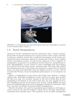
FIGURE 1.1. A high performance robot hand.

Isaac Asimov proposed these four refined laws of "robotics" to protect
us from intelligent generations of robots. Although we are not too far from
that time when we really do need to apply Asimov’s rules, there is no
immediate need however, it is good to have a plan.
The term robotics refers to the study and use of robots. The term was
first adopted by Asimov in 1941 through his short science fiction story,
Runaround.
Based on the Robotics Institute of America (RIA) definition: "A robot is

a reprogrammable multifunctional manipulator designed to move material,
parts, tools, or specialized devices through variable programmed motions
for the performance of a variety of tasks."
R.N. Jazar, Theory of Applied Robotics, 2nd ed., DOI 10.1007/978-1-4419-1750-8_1,
© Springer Science+Business Media, LLC 2010