- Trang chủ >>
- Khoa Học Tự Nhiên >>
- Vật lý
ON PECCEI QUINN SYMMETRY AND QUARK MASSES IN THE ECONOMICAL 3 3 1 MODEL
Bạn đang xem bản rút gọn của tài liệu. Xem và tải ngay bản đầy đủ của tài liệu tại đây (187.84 KB, 16 trang )
Proc. Natl. Conf. Theor. Phys. 37 (2012), pp. 1-16
ON PECCEI-QUINN SYMMETRY AND QUARK MASSES IN THE
ECONOMICAL 3-3-1 MODEL
H. T. HUNG
Department of Physics, Ha Noi University of Educations N0 2, Xuan Hoa, Phuc Yen,
Vinh Phuc, Vietnam
V.T. N. HUYEN, P. V. DONG AND H. N. LONG
Institute of Physics, VAST, P. O. Box 429, Bo Ho, Hanoi 10000, Vietnam
Abstract. We show that there is an infinite number of U (1) symmetries like Peccei-Quinn symmetry in the 3-3-1 model with minimal scalar sector. Moreover, all of them are completely broken
due to the gauge symmetry breaking with the model’s scalars. There is no any residual PecceiQuinn symmetry. Because of the minimal scalar content there are some quarks that are massless
at tree-level, but they can get consistent mass contributions at one-loop due to this fact.
I. INTRODUCTION
There are obvious evidences that we must go beyond the standard model. The
leading questions of which are perhaps neutrino oscillation, natural origin of masses and
particularly Higgs mechanism, hierarchy problem between weak and Planck scale, and
matter-antimatter asymmetry in the universe. In this work we will, however, be interested
in alternatives concerning flavor physics. Why are there just three families of fermions?
How are the families related? What are the nature of flavor mixings and mass hierarchies?
On 3-3-1 models, the gauge symmetry has the form SU (3)C ⊗ SU (3)L ⊗ U (1)X (thus
named 3-3-1). A fermion content satisfying all the requirements is
ψaL = (νa , ea , Nac )TL ∼ (1, 3, −1/3) ,
(u1 , d1 , U )TL
eaR ∼ (1, 1, −1) ,
Q1L =
∼ (3, 3, 1/3) , QαL = (dα , −uα , Dα )TL ∼ (3, 3∗ , 0) ,
uaR , UR ∼ (3, 1, 2/3) , daR , DαR ∼ (3, 1, −1/3),
(1)
where α = {2, 3} and a = {1, α} are family indices. The quantum numbers as given in
parentheses are respectively based on (SU (3)C , SU (3)L , U (1)X ) symmetries. The U and
D are exotic quarks, while NR are right-handed neutrinos. The model is thus named the
3-3-1 model with right-handed neutrinos. If these exotic leptons are not introduced, i.e.
instead the third components are now included right-handed charged leptons, we have the
minimal 3-3-1 model.
The 3-3-1 gauge symmetry is broken through two stages: SU (3)L ⊗ U (1)X −→
SU (2)L ⊗ U (1)Y −→ U (1)em . They are obtained by scalar triplets. One of the weaknesses
of the mentioned 3-3-1 models that reduces their predictive possibility is a plenty or
complication in the scalar sectors. The attempts on this direction to realize simpler scalar
sectors have recently been made. The first one is the 3-3-1 model with right-handed
2
H. T. HUNG, V. T. N. HUYEN, P.V.DONG AND H. N. LONG
neutrinos and minimal scalar sector—two triplets [?],
χ =
0
χ01 , χ−
2 , χ3
T
φ =
0 +
φ+
1 , φ2 , φ3
T
∼ (1, 3, −1/3) ,
∼ (1, 3, 2/3) ,
(2)
with VEV given by
u
1
χ = √ 0 ,
2
ω
0
1
φ = √ v ,
2
0
(3)
called the economical 3-3-1 model [?, ?]. The VEV ω is responsible for the first stage of
gauge symmetry breaking, while v, u are for the second stage. The minimal 3-3-1 model
with minimal scalar sector of two triplets has also been proposed in Ref. [7]. Notice
that due to the restricted scalar contents, these models often contain tree-level massless
quarks that require corrections. The latter model has provided masses for quarks via highdimensional effective interactions, whereas the former one has produced quark masses via
quantum effects.
II. Peccei-Quinn symmetries in economical 3-3-1 model.
The gauge symmetry of the model is SU (3)C ⊗ SU (3)L ⊗ U (1)X . The particle
content is defined in equations (1,2). The electric charge operator is given by
1
Q = T3 − √ T8 + X,
3
(4)
where Ti (i = 1, 2, 3, ..., 8) and X are the charges of SU (3)L and U (1)X ,√respectively. The
standard model hypercharge operator is thus identified as Y = −(1/ 3)T8 + X. This
model does not contain exotic electric charges, i.e. the exotic quarks have electric charges
like ordinary quarks: Q (D) = −1/3 and Q (U ) = 2/3.
The most general Yukawa interactions are given by
∗
LY = hU Q1L χUR + hD
αβ QαL χ DβR
c
+heab ψ aL φebR + hνab ǫmnp (ψ aL )m (ψbL )n (φ)p
+hda Q1L φdaR + huαa QαL φ∗ uaR
+sua Q1L χuaR + sdαa QαL χ∗ daR
U
∗
+sD
α Q1L φDαR + sα QαL φ UR + H.c.,
(5)
where m, n and p stand for SU(3)L indices. In [?] we have shown that at the tree level one
up-quark and two down-quarks are massless. However, the one-loop corrections can give
them consistent masses. In this work we will revisit those corrections by giving a complete
calculation when including a realistic mixing of all the three families of quarks as well. We
are thus showing that the results in [12] which contrast with ours are not correct.
As the lepton triplets stand, the lepton number in this model does not commute
with the gauge symmetry. In fact, it is a residual symmetry of a new-lepton charge L
On Peccei-Quinn symmetry and quark masses in the economical 3-3-1 model
3
given by [?]
4
(6)
L = √ T8 + L.
3
The L charges of the model multiplets can be obtained as
1 2 2 2 4
(7)
L(ψaL , Q1L , QαL , φ, χ, eaR , uaR , daR , UR , DαR ) = , − , , − , , 1, 0, 0, −2, 2,
3 3 3 3 3
respectively. Also, it is easily checked that L(U ) = −L(D) = L(φ3 ) = −L(χ1,2 ) = −2.
All the other quarks and scalars have zero lepton-number, L = 0. It is worth emphasizing
that the residual L is spontaneously broken by u due to L(χ01 ) = 2, which is unlike the
standard model. Notice that the Yukawa couplings s’s violate L, while the h’s do not.
Following [12], we introduce a global U (1)H symmetry in addition to the gauge
symmetry, i.e.
SU (3)C ⊗ SU (3)L ⊗ U (1)X ⊗ U (1)H .
(8)
The condition for this symmetry playing the role like Peccei-Quinn (handedness or chiral)
symmetry is anomaly [SU (3)C ]2 U (1)H = 0. On the other hand, since the Yukawa interactions invariant under this symmetry, the relations on the charges of any U (1)H group
are
−HQ1 + HU + Hχ = 0,
−HQ1 + Hu + Hχ = 0,
−HQ1 + Hd + Hφ = 0,
−HQ1 + HD + Hφ = 0,
−Hψ + He + Hφ = 0,
−HQ + HD − Hχ = 0,
−HQ + Hd − Hχ = 0,
−HQ + Hu − Hφ = 0,
−HQ + HU − Hφ = 0,
2Hψ + Hφ = 0,
(9)
(10)
(11)
(12)
(13)
where the notation HΨ means as the U (1)H charge of the Ψ multiplet. Notice that all
the other terms of Lagrangian are obviously conserved under this symmetry. Using the
relations, the anomaly mentioned is rewritten as
[SU (3)C ]2 U (1)H ∼ 2Hχ + Hφ = 0.
(14)
In solving equations (9-13,14), we also denote H as a collection of partial solutions
HΨ in order, and having remarks as follows
(1) The solution is scale invariance, i.e. if H is solution, then cH (c = 0) does.
(2) Two solutions called to be different (i.e. linearly independent) if they are not
related by scale invariance transformations.
(3) The solutions that contain linearly-independent subsolutions, e.g. (Hφ , Hχ ) =
(0, 1), (1, 0), or (1, 1), respectively, are different.
(4) The different solutions will define different Peccei-Quinn like symmetries, respectively.
The charge relations (9-13) yield degenerate equations. Indeed, they can equivalently be rewritten via seven independent equations as follows
Hu = HU , Hd = HD , Hψ = −Hφ /2, He = −3Hφ /2,
Hu − Hd = Hφ − Hχ , Hu − HQ = Hφ , Hu + Hd = HQ + HQ1 .
(15)
4
H. T. HUNG, V. T. N. HUYEN, P.V.DONG AND H. N. LONG
We have 10 variables, while there are 7 equations. Hence, there is an infinite number of
solutions (certainly satisfying (14) too). For instant, put Hφ = 0. We have Hψ = He = 0,
Hu = HU = HQ , Hd = HD = HQ1 , and Hu − Hd = −Hχ . The solutions of this kind are
thus given dependently on two parameters a ≡ Hχ = 0 and b ≡ Hu such as
H(φ, χ, ψ, e, u, U, Q, d, D, Q1 ) = (0, a, 0, 0, b, b, b, a + b, a + b, a + b).
(16)
Since a, b are arbitrary, there are an infinity of different solutions corresponding to whatever
pairs (a, b) are linearly independent, for example, (a, b) = (0, 1), (1, 0), (1, 1), (1, 2) and
so on.
In Table 1, we list three of Peccei-Quinn like symmetries in which the first one
(second line) is given in [12] that was solely claimed and marked as U (1)P Q .
Table 1. Three chiral symmetries taken as examples in the economical 3-3-1 model.
QαL
−1
1
1
Q1L
1
2
2
(uaR , UR )
0
1
2
(daR , DαR )
ψaL
eaR
0
−1/2 −3/2
2
0
0
1
−1/2 −3/2
φ
1
0
1
χ
1
1
0
There is no residual symmetry associated with the U (1)H above after the spontaneous gauge-symmetry breaking which contradicts with [12]. Prove: suppose that
there is such one, denoted by U (1)P Q . Since it is sevival and conserved after the electroweak symmetry breaking, it has the form as a combination of diagonal generators
P Q = αT3 + βT8 + δX + γH (γ = 0). Also, the charge P Q has to annihilate the vacuums,
P Q( φ , χ ) = 0. All these are similar to the electric charge operator responsible for
electric charge conservation after the electroweak symmetry breaking. We have equations:
α
β
+ √ + δXχ + γHχ = 0,
2
2 3
β
α
− + √ + δXφ + γHφ = 0,
2
2 3
β
− √ + δXχ + γHχ = 0.
3
(17)
Combining all three equations, we deduce δ(2Hχ + Hφ ) = 0. Because 2Xχ + Xφ = 0
If δ = 0 , then 2Hχ + Hφ = 0 that contradicts to (14), [SU (3)C ]2 U (1)H ∼ 2Hχ + Hφ = 0.
Therefore, there is no residual symmetry of U (1)H . All the Peccei-Quinn like U (1)H
symmetries
√ are completely broken along with the gauge symmetry breaking. If δ = 0 then
β = −α/ 3 and γ = α , Therefore we have P Q = αQ as a solution to finding the electric
charge operation (that certainly contradicts to (14) since Q is vectorlike). If one includes
baryon number B as well (since Bφ = Bχ = 0), it results
P Q = αQ + ξB.
(18)
On Peccei-Quinn symmetry and quark masses in the economical 3-3-1 model
5
Only vectorlike symmetries (i.e. non Peccei-Quinn) such as X, B might have surviving
residual symmetries after the spontaneous symmetry breaking by the model’s scalars.
III. Fermion masses .
In this model, the masses of charged leptons are given at the tree level as usual
while the neutrinos can get consistent masses at the one-loop level as explicitly pointed
out in Ref. [19]. The implication of the higher-dimensional effective operators responsible
for the neutrino masses has also been given therein.
Let us now concentrate on masses of quarks that can be divided into two sectors: up
type quarks (ua , U ) with electric charge 2/3 and down type quarks (da , Dα ) with electric
charge −1/3. From (5) and (3) we can obtain the mass matrix of the up type quarks
(u1 , u2 , u3 , U ):
−su1 u −su2 u −su3 u −hU u
1 hu21 v hu22 v hu23 v
sU
2 v ,
(19)
Mup = √
u
u
u
U
s3 v
2 h31 v h32 v h33 v
−su1 ω −su2 ω −su3 ω −hU ω
and the mass matrix of down type quarks
d
h1 v
sd21 u
1 d
s31 u
Mdown = − √
2
sd ω
21
sd31 ω
(d1 , d2 , d3 , D2 , D3 ):
hd2 v
sd22 u
sd32 u
sd22 ω
sd32 ω
hd3 v
sd23 u
sd33 u
sd23 ω
sd33 ω
sD
2 v
hD
22 u
hD
32 u
hD
22 ω
hD
32 ω
sD
3 v
hD
23 u
hD
33 u
hD
23 ω
hD
33 ω
.
(20)
The first and last rows of (19) are proportional. Similarly, the second and fourth rows of
(20) are proportional, while the third and last rows of this matrix take the same situation.
Hence, in this model the tree level quark spectrum contains three massless eigenstates
(one up and two down quarks). So, what are the causes?
There are just two: first all these degeneracies are due to the χ scalar only (with
the presence of VEVs u, ω), not φ; second, the Yukawa couplings of the first and third
component of quark triplets/antitriplets to right-handed quarks in those degenerate rows
are the same due to SU (3)L invariance. Obviously, the vanishing quark masses are not a
consequence of the U (1)H symmetry because it actually happens even if we choose Hχ = 0
(in this case the Peccei-Quinn like symmetry resulting from only Hφ = 0 does not give
any constraint on the massless quark sector). At the one-loop level, all the degeneracies
will be separated due to contribution of φ as well (see Appendix B of [8]). In such case,
the one-loop mass corrections also collectively break the U (1)H symmetry since both the
scalars χ, φ are being taken into account, i.e. for those relevant quarks 2Hχ + Hφ are
always nonzero at the one loop level.
In [8], we have already shown that all the tree level massless quarks can get consistent
masses at the one-loop level. There, the light quarks and/or mixings of light quarks with
exotic quarks got mass contributions. The exotic quark masses are reasonably large and
took as a cutoff scale, thus no correction is needed. So why the recalculations as given in
6
H. T. HUNG, V. T. N. HUYEN, P.V.DONG AND H. N. LONG
Ref. [12] for the quark masses, that consequently contradict to ours, are incomplete? This
is due to the fact that they included even mass corrections for heavy exotic quarks as well.
In this case, the cutoff scale of the theory must be larger than the exotic quark masses. As
a result, under this cutoff scale all the physics is sensitive. There must be contributions
coming from the φ scalar as well as ordinary active quarks where the flavor mixing must
present. Let us remind that Ref. [12] in this case accounts for the χ contribution only.
Thus the masslessness would remain as a result of two points mentioned above.
The above analysis also means that all quarks will get masses if both χ and φ
contribute so that 2Hχ + Hφ = 0 to ensure (14). This can explicitly be understood via an
analysis of the effective mass operators [13] responsible for quarks below.
III.1. One-loop corrections
The analysis given below is for the up type quark sector only. That for the down
type quark sector can be done similarly and got the same conclusion as the up type quarks.
After the one-loop corrections, the mass matrix (19) looks like
−su1 u + ∆11 −su2 u + ∆12 −su3 u + ∆13 −hU u + ∆14
1 hu21 v + ∆21 hu22 v + ∆22 hu23 v + ∆23
sU
2 v + ∆24 ,
(21)
Mup = √
U
u
u
u
s3 v + ∆34
h31 v + ∆31 h32 v + ∆32 h33 v + ∆33
2
−su1 ω + ∆41 −su2 ω + ∆42 −su3 ω + ∆43 −hU ω + ∆44
where ∆ij are all possible one-loop corrections. Obviously this matrix gives all nonzero
masses if the first and last rows are not in proportion. To show that tree-level degeneracy
separated (i.e. these two rows are now not proportional) it is only necessary to prove the
following submatrix:
1
MuU = √
2
−su1 u + ∆11 −hU u + ∆14
−su1 ω + ∆41 −hU ω + ∆44
(22)
having nonzero determinant with general Yukawa couplings and VEVs. Two conditions
below should be clarified: (i) The tree-level properties as implemented by the two points
above must be broken,
∆11
∆14
∆41
∆44
=
=
su
1
hU
su
1
hU
∆11
∆41
∆14
∆44
=
=
u
ω
u
ω
,
.
(23)
(24)
Since, by contrast if one of these systems is unsatisfied, which is the case as analyzed in
[12], one quark remains massless. (ii) The matrix (22) has nonzero determinant:
detMuU
=
or
1 u
s (ω∆14 − u∆44 ) + hU (u∆41 − ω∆11 ) + ∆11 ∆44 − ∆41 ∆14 = 0 (25)
2 1
1
(26)
u(hU ∆41 − su1 ∆44 ) + ω(su1 ∆14 − hU ∆11 ) + ∆11 ∆44 − ∆41 ∆14 = 0.
2
It is interesting that the first two terms of (25) and (26) mean (24) and (23), respectively.
On Peccei-Quinn symmetry and quark masses in the economical 3-3-1 model
7
At the one loop level, there must be similar corrections mediated coming from
ordinary quarks, exotic quarks as well as both ordinary and exotic quarks in mediations.
We must also include general Yukawa couplings connecting flavors, i.e. hab = 0, sab = 0
for a = b to account for the CKM quark mixing matrix as it should be. It is also remarked
that the external scalar lines of those diagrams now consist of φ, χ or both χ and φ as
well. Totally, we have 48 diagrams at the one-loop level (24 for up type quark and 24 for
down type quark). See Appendix B of [8] for details. Here, for a convenience let us list
all those corrections in terms of the relevant matrix elements as given in Appendix B. All
the one-loop corrections are taken into account to yield (22) explicitly
∆11 =
∆41 =
huα1
sU
α
huα1
sU
α
4
∆i14 +
i=1
4
∆i44 +
i=1
su1
hU
su1
hU
8
8
∆j14 ,
∆14 =
j=5
∆k14 ,
(27)
∆k44 .
(28)
k=1
8
8
∆j44 ,
∆44 =
j=5
k=1
It is easily checked that (23) is satisfied since
huα1
su1
=
,
sU
hU
α
huα1 = 0,
sU
α = 0,
(29)
in general. This is due to the contribution of φ to the massless quarks (in addition to
χ) as well like we can already see from the Yukawa couplings huα1 and sU
α related to this
scalar. The system (24) is always correct even we can check that it is also applied for the
special case with flavor diagonalization as presented in [8, 12].
Finally let us check (ii). The determinant equals to
detMup
1
=
2
su1
huα1
−
sU
hU
α
hU
4
4
i=1
(u∆i44 − ω∆i14 ) +
8
i=1 j=5
(∆i14 ∆j44 − ∆j14 ∆i44 ) , (30)
8
H. T. HUNG, V. T. N. HUYEN, P.V.DONG AND H. N. LONG
which is always nonzero due to (29). In fact, the last factor [· · · ] can be explicitly given
by
2
2
2
, Md2i , Mφ23 ) + I(MQ
hU [(ω 2 + u2 )λ3 + u2 λ4 + v 2 λ2 ][u[I(MQ
, MD
, Mφ23 )]
α
α1,3
α1,3
2
2
2
2
2
2
2
− ω[I(MQ
, Md2i , Mφ21 ) + I(MQ
, MD
, Mφ21 )] + Mχ23 u[B(MQ
2 , Mdi , Mχ2 , Mφ3 )
α
α1,3
α1,3
1
2
2
2
2
2
2
2
2
2
2
2
2
2
+B(MQ
2 , MDα , Mχ2 , Mφ3 )] − Mχ1 ω[B(MQα2 , Mui , Mφ2 , Mχ1 ) + B(MQα2 , MU , Mφ2 , Mχ1 )]
1
2
2
2
, Mu2i , Mφ23 ) + Mφ21 B(MQ
, Md2i , Mφ23 , Mφ21 )
− (ω − u)uω[A(MQ
, Md2i , Mφ23 ) + A(MQ
α2
α1,3
α1,3
2
2
2
, Mu2i , Mφ23 )
+Mφ21 B(MQ
, Mu2i , Mφ23 , Mφ21 )]] + uω[A(MQ
, Md2i , Mφ23 ) + A(MQ
α2
α2
α1,3
2
2
, Mu2i , Mφ23 , Mφ21 )] [[((ω 2 + u2 )λ1 + v 2 λ3 )
+ Mφ21 B(MQ
, Md2i , Mφ23 , Mφ21 ) + Mφ21 B(MQ
α2
α1,3
2
2
2
2
2
2
2
2
2
2
2
2
×[(I(MQ
1,3 , MU , Mχ1 ) + I(M 1,3 , Mui , Mχ1 )) − (I(M 1,3 , MU , Mχ3 ) + I(M 1,3 , Mui , Mχ3 ))]]
Q
Q
Q
1
1
1
1
2
2
2
, Mu2i , Mφ22 , Mχ21 )
, MU2 , Mφ22 ) + Mχ21 [B(MQ
+u[A(MQ
, Mu2i , Mφ22 ) + A(MQ
α2
α2
α2
2
2
2
2
2
2
2
+B(MQ
, MU2 , Mφ22 , Mχ21 )]] − ω[A(MQ
2 , Mdi , Mχ2 ) + A(MQ2 , MDα , Mχ2 )]
α2
1
1
2
2
2
2
2
2
2
2
2
2
2
+Mφ23 [B(MQ
2 , Mdi , Mχ2 , Mφ3 ) + B(MQ2 , MDα , Mχ2 , Mφ3 )]]] + uω[A(MU , MU , Mχ3 )
1
1
+A(MU2 , Mu2i , Mχ23 ) + Mχ21 B(MU2 , MU2 , Mχ23 , Mχ21 ) + Mχ21 B(MU2 , Mu2i , Mχ23 , Mχ21 )]
2
2
2
×[[(ω 2 + u2 )λ3 + u2 λ4 + v 2 λ2 ][(I(MQ
, Md2i , Mφ23 ) + I(MQ
, MD
, Mφ23 ))
α
α1,3
α1,3
2
2
2
2
2
−(I(MQ
, Md2i , Mφ21 ) + I(MQ
, MD
, Mφ21 ))] + ω[A(MQ
, Mu2i , Mφ22 ) + A(MQ
, MU2 , Mφ22 )
α
α1,3
α1,3
α2
α2
2
2
2
+Mχ23 [B(MQ
, Mu2i , Mφ22 , Mχ23 ) + B(MQ
, MU2 , Mφ22 , Mχ23 )]] − u[A(MQ
, Mu2i , Mφ22 )
α2
α2
α2
2
2
2
, MU2 , Mφ22 , Mχ21 )]]]
, Mu2i , Mφ22 , Mχ21 ) + B(MQ
+A(MQ
, MU2 , Mφ22 ) + Mχ21 [B(MQ
α2
α2
α2
2
2
2
+{[(ω 2 + u2 )λ3 + u2 λ4 + v 2 λ2 ][I(MQ
, Md2i , Mφ21 ) + I(MQ
, MD
, Mφ21 )]
α
α1,3
α1,3
2
2
2
, Mu2i , Mφ22 , Mχ21 )
, MU2 , Mφ22 ) + Mχ21 [B(MQ
+u A(MQ
, Mu2i , Mφ22 ) + A(MQ
α2
α2
α2
2
2
2
2
2
2
2
+B(MQ
, MU2 , Mφ22 , Mχ21 )] }{[(ω 2 + u2 )λ1 + v 2 λ3 ][I(MQ
1,3 , MU , Mχ3 ) + I(M 1,3 , Mui , Mχ3 )]
α2
Q
1
+ω
2
2
2
A(MQ
2 , Mdi , Mχ2 ) +
1
2
2
2
A(MQ
2 , MDα , Mχ2 )
1
+
1
2
2
2
2
Mφ23 [B(MQ
2 , Mdi , Mχ2 , Mφ3 )
1
2
2
2
2
2
2
2
2
2
2
2
2
2
+B(MQ
2 , MDα , Mχ2 , Mφ3 )] } − {[(ω + u )λ1 + v λ3 ][I(M 1,3 , MU , Mχ1 ) + I(M 1,3 , Mui , Mχ1 )]
Q
Q
1
+u
2
2
2
A(MQ
2 , Mdi , Mχ2 ) +
1
1
2
2
2
A(MQ
2 , MDα , Mχ2 )
1
+
1
2
2
2
2
Mφ21 [B(MQ
2 , Mdi , Mχ2 , Mφ1 )
1
2
2
2
2
2
2
2
2
2
2
2
+B(MQ
2 , MDα , Mχ2 , Mφ1 )] }{[(ω + u )λ3 + u λ4 + v λ2 ][I(MQα1,3 , Mdi , Mφ1 )
1
2
2
, Mφ21 )] +
+I(MQ
, MD
α
α1,3
2
2
, MU2 , Mφ22 )
u A(MQ
, Mu2i , Mφ22 ) + A(MQ
α2
α2
2
2
+ Mχ21 [B(MQ
, Mu2i , Mφ22 , Mχ21 ) + B(MQ
, MU2 , Mφ22 , Mχ21 )] },
α2
α2
where the functions I, A and B are defined in Appendix A. We conclude that all the
quarks in this model can get nonzero masses at the one-loop level. Although the tree level
(31)
On Peccei-Quinn symmetry and quark masses in the economical 3-3-1 model
9
vanishing masses of quarks is not a consequence of the U (1)H symmetry, this Peccei-Quinn
like symmetry is collectively broken at the one-loop level when the quarks get masses.
III.2. Effective mass operators
As previous section, the U (1)H symmetry is spontaneously broken via the collective
effects at the one-loop level when all the quarks get mass, i.e. 2Hχ +Hφ = 0. In this section,
we will show that all the quarks can get mass via effective mass operators there the U (1)H
breaking is explicitly recognized. In other words, we will consider effective interactions
responsible for fermion masses up to five dimensions. The most general interactions up to
five dimensions that lead to fermion masses have the form:
LY + L′Y ,
(32)
where LY is defined in (5) and L′Y (five-dimensional effective mass operators) is given by
L′Y
=
1
(Q φ∗ χ∗ )(s′U UR + h′u
a uaR )
Λ 1L
1
′d
+ (QαL φχ)(s′D
αβ DβR + hαa daR )
Λ
1
c
+ s′ν
(ψ ψbL )(χχ)∗
Λ ab aL
+H.c.
(33)
Here, as usual we denote h for L-charge conservation couplings and s for violating ones. Λ
is the cutoff scale which can be taken in the same order as ω. It is noteworthy that all the
above interactions (as given in L′Y ) are not invariant under U (1)H since they carry U (1)H
charge proportional to 2Hχ +Hφ = 0 like (14). For example, the first interaction has U (1)H
charge: −HQ1 − Hφ − Hχ + Hu = −(2Hχ + Hφ ), with the help of eqs (9-13). All those
interactions contain φχ combination. Therefore, the fermion masses are generated if both
scalars develop VEV. In this case, the Peccei-Quinn like symmetry U (1)H is spontaneously
broken too.
Substituting VEVs (3) into (32), the mass Lagrangian reads
T
Lmass
f ermion = −(u1L u2L u3L U L )Mu (u1R u2R u3R UR )
−(d1L d2L d3L D 2L D 3L )Md (d1R d2R d3R D2R D3R )T
1
− (ν cL N R )Mν (νL NRc )T
2
+H.c.
(34)
Here the mass matrices of up type quarks (u1 u2 u3 U ), down type quarks (d1 d2 d3 D2 D3 )
are respectively given by
′u −su u − √1 vω h′u −su u − √1 vω h′u −hU u − √1 vω s′U
−su1 u − √12 vω
2
3
Λ h1
2 Λ 2
2 Λ 3
2 Λ
1
sU
hu23 v
hu22 v
hu21 v
2v
Mu = √
,
u v
u v
u v
Uv
h
h
h
s
2
31
32
33
3
′u −su ω + √1 vu h′u −su ω + √1 vu h′u −hU ω + √1 vu s′U
h
−su1 ω + √12 vu
2
3
Λ 1
2 Λ 2
2 Λ 3
2 Λ
(35)
10
H. T. HUNG, V. T. N. HUYEN, P.V.DONG AND H. N. LONG
−1
Md = √
2
hd1 v
′d
sd21 u + √12 vω
Λ h21
1
vω
d
s31 u + √2 Λ h′d
31
′d
sd21 ω − √12 vu
h
Λ 21
′d
sd31 ω − √12 vu
Λ h31
hd2 v
′d
sd22 u + √12 vω
Λ h22
1
vω
d
s32 u + √2 Λ h′d
32
′d
sd22 ω − √12 vu
h
Λ 22
′d
sd32 ω − √12 vu
Λ h32
hd3 v
′d
sd23 u + √12 vω
Λ h23
1
vω
d
s33 u + √2 Λ h′d
33
′d
sd23 ω − √12 vu
h
Λ 23
′d
sd33 ω − √12 vu
Λ h33
sD
sD
3 v
2 v
1
vω
D
′D
D
′D
√
h22 u + 2 Λ s22 h23 u + √12 vω
Λ s23
1
1
vω
vω
D
′D
D
h32 u + √2 Λ s32 h33 u + √2 Λ s′D
33
√1 vu s′D hD ω − √1 vu s′d
ω
−
hD
22
23
2 Λ 22
2 Λ 23
√1 vu s′D hD ω − √1 vu s′D
ω
−
hD
32
33
2 Λ 32
2 Λ 33
(36)
Two remarks are in order
(1) Up quarks: If there is no correction, i.e. s′ , h′ = 0, the mass matrix (35) has
the first line and the fourth line in proportion (degeneracy) that means that
one up quark is massless, as mentioned [8]. The presence of corrections, i.e.
s′ , h′ = 0, will separate that degeneracy. Indeed, the first and fourth lines are
U ′U which is not the
′u
u
′u
u
now in proportion only if su1 /h′u
1 = s2 /h2 = s3 /h3 = h /s
case in general. The up quark type mass matrix is now most general that can
be diagonalized to obtain the masses of exotic U and ordinary u1,2,3 .
(2) Down quarks: The second and the fourth lines as well as the third and the
fifth lines have the same status as in the up quark type. All these degeneracies
are separated. Consequently we have the most general mass matrix for down
quark type.
Using the U (1)H violating triple scalar interactions as mentioned above, those effective
mass operators with five dimensions can be explicitly understood as derived from two-loop
radiative corrections responsible for the quark masses, with the assumption that U (1)H
was broken in the scalar potential first, in similarity to the radiative Majorana neutrino
masses via lepton violating triple scalar potentials in Zee-Babu model [20]. It is noted
that the above one-loop corrections can be also translated via the language of effective
operators with six dimensions before the U (1)H breaking happens. A complete calculation
of all the corrections presented above as well as obtaining the quark masses and mixing is
out of scope of this work. It should be published elsewhere [21].
IV. CONCLUSION
V. Conclusions
As any other 3-3-1 models, the economical 3-3-1 model naturally contains an infinity
of U (1)H symmetries like Peccei-Quinn symmetry with just its scalar content, which is
unlike the case of the standard model. In contradiction to other extensions of the standard
model including ordinary 3-3-1 models, the economical 3-3-1 model has interesting features
as follows
(1) There is no residual symmetry of U (1)H after the scalars getting VEVs.
(2) The vanishing of quark masses at the tree-level is not a resultant from U (1)H .
It is already a consequence of the minimal scalar content under the model
gauge symmetry.
(3) All the quarks can get nonzero masses at the one-loop level, there the U (1)H
symmetry is obviously broken.
.
On Peccei-Quinn symmetry and quark masses in the economical 3-3-1 model
11
By this work, it is to emphasis that the economical 3-3-1 model can work with only
two scalar triplets. All the fermions can get consistent masses [8, 19]. A further analysis
can show observed flavor mixings as indicated by the CKM matrix and PMNS matrix.
Also, with the minimal scalar sector the model is very predictive which is worth to be
searched for at the current colliders [21].
With the above conclusions, it is to emphasis that the statements in [12] such as
unique solution of U (1)H , existence of a residual symmetry of U (1)H , the masslessness
of quarks due to that supposed residual symmetry, and one loop corrections to up type
quark sector are incorrect or incomplete. The addition of scalars to the economical 3-3-1
model as given in [12] is dynamically not required since this model as seen can work well
by itself.
REFERENCES
[1] K. Nakamura et al. [Particle Data Group], J. Phys. G 37, 075021 (2010), and references therein.
[2] P. Langacker, Phys. Rept. 72, 185 (1981), and references therein.
[3] See, for examples, A. Doff and F. Pisano, Mod. Phys. Lett. A 15, 1471 (2000); P. V. Dong and H. N.
Long, Int. J. Mod. Phys. A 21 6677, (2006).
[4] M. Singer, J. W. F. Valle and J. Schechter, Phys. Rev. D 22, 738 (1980); J. C. Montero, F. Pisano
and V. Pleitez, Phys. Rev. D 47, 2918 (1993); R. Foot, H. N. Long and Tuan A. Tran, Phys. Rev. D
50, 34(R) (1994); H. N. Long, Phys. Rev. D 53, 437 (1996); 54, 4691 (1996).
[5] F. Pisano and V. Pleitez, Phys. Rev. D 46, 410 (1992); P. H. Frampton, Phys. Rev. Lett. 69, 2889
(1992); R. Foot, O. F. Hernandez, F. Pisano and V. Pleitez, Phys. Rev. D 47, 4158 (1993).
[6] W. A. Ponce, Y. Giraldo and L. A. Sanchez, Phys. Rev. D 67, 075001 (2003); P. V. Dong, H. N. Long,
D. T. Nhung and D. V. Soa, Phys. Rev. D 73, 035004 (2006); P. V. Dong and H. N. Long, Adv. High
Energy Phys. 2008, 739492 (2008).
[7] J. G. Ferreira, Jr, P. R. D. Pinheiro, C. A. de S. Pires and P. S. Rodrigues da Silva, Phys. Rev. D 84,
095019 (2011)
[8] P. V. Dong, Tr. T. Huong, D. T. Huong, and H. N. Long, Phys. Rev. D 74, 053003 (2006).
[9] P. B. Pal, Phys. Rev. D 52, 1629 (1995); C. A. de S. Pires and O. P. Ravinnez, Phys. Rev. D 58,
035008 (1998); C. A. de S. Pires, Phys. Rev. D 60, 075013 (1999).
[10] R. D. Peccei and H. R. Quinn, Phys. Rev. Lett. 38, 1440 (1977); Phys. Rev. D 16, 1791 (1977).
[11] S. Weinberg, Phys. Rev. Lett. 40, 223 (1978); F. Wilczek, Phys. Rev. Lett. 40, 279 (1978).
[12] J. C. Montero and B. L. Sanchez-Vega, Phys. Rev. D 84, 055019 (2011).
[13] S. Weinberg, Phys. Rev. Lett. 43, 1566 (1979); F. Wilczek and A. Zee, Phys. Rev. Lett. 43, 1571
(1979).
[14] Y. Chikashige, R. N. Mohapatra, and R. D. Peccei, Phys. Lett. B 98, 265 (1981); G. B. Gelmini and
M. Roncadelli, Phys. Lett. B 99,411 (1981).
[15] D. Chang and H. N. Long, Phys. Rev. D 73, 053006 (2006).
[16] P. V. Dong, H. N. Long, and D. V. Soa, Phys. Rev. D 73, 075005 (2006).
[17] L. N. Epele, H. Fanchiotti, C. G. Canal, and W. A. Ponce, arXiv:hep-ph/0701195.
[18] P. V. Dong, L. T. Hue, H. N. Long, and D. V. Soa, Phys. Rev. D 81, 053004 (2010); P. V. Dong, H.
N. Long, D. V. Soa, and V. V. Vien, Eur. Phys. J. C 71, 1544 (2011); P. V. Dong, H. N. Long, C. H.
Nam, and V. V. Vien, Phys. Rev. D 85, 053001 (2012).
[19] P. V. Dong, H. N. Long, and D. V. Soa, Phys. Rev. D 75, 073006 (2007).
[20] A. Zee, Nucl. Phys. B 264, 99 (1986); K. S. Babu, Phys. Lett. B 203, 132 (1988).
[21] P. V. Dong, H. T. Hung, and H. N. Long, Question of Peccei-Quinn symmetry and quark masses in
economical 3-3-1 model, Phys. Rev. D 86, 033002 (2012).
12
H. T. HUNG, V. T. N. HUYEN, P.V.DONG AND H. N. LONG
Appendix A. Integrations
The functions A(a, b, c), B(a, b, c, d) and I(a, b, c) as appeared in the text are given
by
A(a, b, c) ≡
=
B(a, b, c, d) ≡
=
I(a, b, c) ≡
=
1
d4 p
(2π)4 (p2 − a)(p2 − b)(p2 − c)
−i
a ln a
b ln b
c ln c
+
+
,
2
16π
(a − b)(a − c) (b − a)(b − c) (c − b)(c − a)
1
d4 p
4
2
2
(2π) (p − a)(p − b)(p2 − c)(p2 − d)
−i
a ln a
b ln b
+
2
16π
(a − b)(a − c)(c − d) (b − a)(b − c)(b − d)
d ln d
c ln c
+
+
,
(c − b)(c − a)(c − d) (d − b)(d − a)(d − c)
p2
d4 p
(2π)4 (p2 − a)2 (p2 − b)(p2 − c)
−i
a(2 ln a + 1)
a2 (2a − b − c) ln a
b2 ln b
−
+
16π 2 (a − b)(a − c)
(a − b)2 (a − c)2
(b − a)2 (b − c)
2
c ln c
+
.
(c − a)2 (c − b)
(37)
(38)
(39)
Appendix B. Corrections
The one-loop corrections to the mass matrix MuU are presented by the diagrams as
follows:
Received 30-09-2012.
On Peccei-Quinn symmetry and quark masses in the economical 3-3-1 model
2
χ1,3
0 , φ0
×
χ01,3 , φ02
×
χ10
×
λ2,3,4
φ1,3
huα1 Qα1,3L
hdi
diR
u1L
uiR
huα1 Qα2L
+
(a) ∆111 (huα1 , hdi , φ1,3
+ , φ1 )
1,3
0
χ1,3 , φ02
χ0 , φ20
×
χ10
×
×
λ2,3,4
DαR sD
α
u1L
u1R
huα1 Qα2L
×
×
λ1,3
Q1,3
1L
φ1
λe
UR
hU
u1L
u1R
su1 Q21L
×
u1R
×
λ1,3
u1L
λ4
χ2
χ1
φ1
λe
uiR
sui
u1L
u1R
su1
Q21L
× χe
(g)
sdi
+
(f) ∆611 (su1 , hdi , χ−
2 , φ1 )
χ10
φ20
×
×
λe
Q1,3
1L
diR
× χe
× χe
su1
u1L
λ4
χ2
χ1
(e) ∆511 (su1 , hU , χ01,3 , χ01 )
2
2
χ1,3
χ1,3
0 , φ0
0 , φ0
χ1,3
hU
(d) ∆411 (huα1 , hU , φ20 , χ01 )
χ10
φ20
×
×
λe
su1
UR
× χe
1,3
+
(c) ∆311 (huα1 , sD
α , φ+ , φ1 )
1,3
1,3
2
χ0 , φ0
χ0 , φ20
u1R
χ1
λe
× χe
χ1,3
φ02
×
λ3
φ2
φ1
huα1 Qα1,3L
u1L
(b) ∆211 (huα1 , sui , φ20 , χ01 )
λe
u1R
sui
uiR
× χe
× χe
φ1,3
χ1
λe
λe
u1R
φ02
×
λ3
φ2
φ1
13
DαR sD
α
× χe
∆711 (su1 , sui , χ01,3 , χ01 )
(h)
−
+
∆811 (su1 , sD
α , χ2 , φ1 )
Fig. 1. Corrections to (MuU )11
u1L
14
H. T. HUNG, V. T. N. HUYEN, P.V.DONG AND H. N. LONG
2
χ1,3
0 , φ0
×
χ01,3 , φ02
×
χ10
×
λ2,3,4
φ1,3
φ2
φ1
sU
α Qα1,3L
hdi
diR
u1L
UR
×
(b)
×
λ2,3,4
φ2
φ1
DαR sD
α
×
u1L
UR
χ2
χ1
UR
×
hU
u1L
UR
×
λ4
φ1
2
hU Q1L
hdi
diR
u1L
× χe
(f)
×
+
∆614 (hU , hdi , χ−
2 , φ1 )
χ10
φ20
×
λ1,3
χ2
χ1
×
λ4
φ1
λe
λe
uiR
sui
u1L
UR
2
hU Q1L
× χe
(g)
u1L
λe
× χe
1,3
hU Q1L
hU
× χe
(e) ∆514 (hU , hU , χ01,3 , χ01 )
2
2
χ1,3
χ1,3
0 , φ0
0 , φ0
UR
UR
×
λ1,3
χ1,3
χ1
U
2
0
(d) ∆414 (sU
α , h , φ0 , χ1 )
χ10
φ20
×
Q1,3
1L
hU
λ3
sU
α Qα2L
λe
UR
×
λe
× χe
+
3
U D
(c) ∆14 (sα , sα , φ1,3
+ , φ1 )
2
2
χ1,3
χ1,3
0 , φ0
0 , φ0
χ1,3
u1L
× χe
×
sU
α Qα1,3L
sui
u
2
0
∆214 (sU
α , si , φ0 , χ1 )
χ10
φ02
λe
UR
χ1
uiR
sU
α Qα2L
× χe
1,3
+
d
(a) ∆114 (sU
α , hi , φ+ , φ1 )
2
χ01,3 , φ02
χ1,3
0 , φ0
φ1,3
λ3
λe
λe
UR
φ02
×
DαR sD
α
× χe
∆714 (hU , sui , χ01,3 , χ01 )
(h)
−
+
∆814 (hU , sD
α , χ2 , φ1 )
Fig. 2. Corrections to (MuU )12 .
u1L
On Peccei-Quinn symmetry and quark masses in the economical 3-3-1 model
2
χ1,3
0 , φ0
×
χ01,3 , φ02
×
χ30
×
λ2,3,4
φ1,3
φ2
φ3
huα1 Qα1,3L
hdi
diR
UL
u1R
×
(b)
×
×
λ2,3,4
φ2
φ3
DαR sD
α
×
su1
UL
u1R
(d)
UR
×
hU
UL
u1R
UL
×
λ4
φ3
su1 Q21L
sdi
diR
UL
× χe
(f)
×
+
∆641 (su1 , hdi , χ−
2 , φ3 )
χ30
φ20
×
λ1,3
χ2
χ3
λe
×
λ4
φ3
λe
uiR
sui
UL
u1R
su1 Q21L
DαR sD
α
× χe
× χe
(g)
hU
λe
× χe
su1 Q1,3
1L
UR
∆441 (huα1 , hU , φ20 , χ03 )
χ30
φ20
χ2
χ3
(e) ∆541 (su1 , hU , χ01,3 , χ03 )
2
2
χ1,3
χ1,3
0 , φ0
0 , φ0
u1R
χ3
×
λ1,3
χ1,3
λ3
× χe
×
Q1,3
1L
×
huα1 Qα2L
λe
u1R
UL
λe
× χe
+
3
u
D
(c) ∆41 (hα1 , sα , φ1,3
+ , φ3 )
2
2
χ1,3
χ1,3
0 , φ0
0 , φ0
χ1,3
sui
uiR
∆241 (huα1 , sui , φ20 , χ03 )
χ30
φ02
λe
u1R
χ3
× χe
+
(a) ∆141 (huα1 , hdi , φ1,3
+ , φ3 )
2
χ01,3 , φ02
χ1,3
0 , φ0
huα1 Qα1,3L
λ3
huα1 Qα2L
× χe
φ1,3
φ02
×
λe
λe
u1R
15
∆741 (su1 , sui , χ01,3 , χ03 )
(h)
−
+
∆841 (su1 , sD
α , χ2 , φ3 )
Fig. 3. Corrections to (MuU )21 .
UL
16
H. T. HUNG, V. T. N. HUYEN, P.V.DONG AND H. N. LONG
2
χ1,3
0 , φ0
×
χ01,3 , φ02
×
χ30
×
λ2,3,4
φ1,3
φ2
φ3
sU
α Qα1,3L
hdi
diR
UL
UR
×
λ2,3,4
φ2
φ3
DαR sD
α
UL
UR
×
sU
α Qα2L
×
×
λ1,3
Q1,3
1L
χ2
χ3
UR
hU
UL
UR
×
φ3
hdi
diR
UL
× χe
(f)
×
×
λ1,3
χ2
χ3
×
λ4
φ3
λe
uiR
sui
UL
UR
2
hU Q1L
× χe
(g)
λ4
+
∆644 (hU , hdi , χ−
2 , φ3 )
χ30
φ20
λe
1,3
hU Q1L
UL
×
2
hU Q1L
× χe
UR
hU
λe
(e) ∆544 (hU , hU , χ01,3 , χ03 )
2
2
χ1,3
χ1,3
0 , φ0
0 , φ0
χ1,3
UR
U
2
0
(d) ∆444 (sU
α , h , φ0 , χ3 )
χ30
φ20
λe
hU
χ3
× χe
× χe
+
3
U D
(c) ∆44 (sα , sα , φ1,3
+ , φ3 )
2
2
χ1,3
χ1,3
0 , φ0
0 , φ0
UR
λ3
λe
λe
χ1,3
UL
u
2
0
(b) ∆244 (sU
α , si , φ0 , χ3 )
3
χ0
φ02
×
×
×
sU
α Qα1,3L
sui
× χe
1,3
+
d
(a) ∆144 (sU
α , hi , φ+ , φ3 )
2
χ01,3 , φ02
χ1,3
0 , φ0
UR
χ3
uiR
sU
α Qα2L
× χe
φ1,3
λ3
λe
λe
UR
φ02
×
DαR sD
α
× χe
∆744 (hU , sui , χ01,3 , χ03 )
(h)
−
+
∆844 (hU , sD
α , χ2 , φ3 )
Fig. 4. Corrections to (MuU )22 .
UL