Inverse modeling for the study of 2d doping profile of submicron transistor using process and device simulation
Bạn đang xem bản rút gọn của tài liệu. Xem và tải ngay bản đầy đủ của tài liệu tại đây (1.01 MB, 112 trang )
Inverse modeling for the study of 2D doping profile
of submicron transistor using process and device
simulation
Chan Yin Hong
National University of Singapore
2005
Inverse modeling for the study of 2D doping profile
of submicron transistor using process and device
simulation
Submitted by
CHAN YIN HONG
(B.Eng.(Hons.), NUS)
A THESIS SUBMITTED
FOR THE DEGREE OF MASTER OF ENGINEERING
DEPARTMENY OF ELECTRICAL AND COMPUTER ENGINEERING
NATIONAL UNIVERSITY OF SINGAPORE
2005
1
ABSTRACT
Direct quantitative determination of 2D doping profile of submicron
MOSFETs continues to be elusive. This project develops a technique to deduce 2D
doping profile by the inverse modeling method combining process and device
simulation.
Based on previous inverse modeling research, this project extends the
inverse modeling technique by including process and device simulation together
with multiple transistors electrical data used as target for matching. Such
methodology will allow a physical way of taking sensitive process steps such as
implantation and high temperature annealing into account. By combining electrical
data like sub-threshold Id-Vg of multiple transistors for matching, the chance of
getting a non-unique solution is kept to minimum. An algorithm which spreads
process simulation to multiple processors is developed to make the time consuming
process simulation more efficient.
Since the final doping profile is based on simulation of doping activation
and diffusion, instead of pure mathematical representation of doping profile as it
was done in the past, the result can be predictive in nature. A set of parameters
obtained can be used for transistors produced with similar technology and process
condition. This allows fast characterization of multiple transistors without the
repeated use of time consuming inverse modeling exercise and provides alternative
to verify the uniqueness of solution obtained.
1
ACKNOWLEDGEMENTS
First and foremost, I would like to express my sincere gratitude to Professor
Chor Eng Fong and Professor Ganesh Samudra, my thesis supervisors, for their
exceptional guidance, continuous encouragement and warm support. Their insights
in research work help me to overcome many hurdles in this project and without
them, this project will not be possible.
I am also indebted to Dr Lap Chan and Dr Francis Benistant who spends
much of valuable time in this project even after a day of hard work in CSM. For
personnel who held responsibility in the corporate world, it must be difficult and
demanding to assign additional time and energy to supervise this academic
activity.
Also, I would like to thanks CSM (Chartered Semiconductor Manufacturer)
for the supportive material they provided me with. Without their test wafer and
extensive hardware/software support, many tests involved in this project would not
be possible. Finally I would like to complement Professor Dimitri A. Antoniadis
and Dr Ihsan J.Djomehri of MIT for their kind help and useful discussion when I
was in United States.
2
CONTENTS
Abstract
1
Acknowledgement
2
Contents
3-5
List of figures
6-8
List of tables
9
List of symbols and abbreviations
10-11
Chapter one – Introduction
12
1.1 Motivation and aim
12-14
1.2 Previous work done using Inverse modeling technique
14-18
1.3 New inverse modeling approach to be examined in this
project
18-22
1.4 Organization of the thesis
22-23
Chapter two – Theory
24
2.1 Physical models in process simulation
24-27
2.1.1 Implantation model selection and modification
27-33
2.1.2 Diffusion model selection
33-37
2.2 Physics behind device simulation
37-41
2.3 Selection of optimizing parameters
41-43
2.4 Selection of matching electrical data
43
2.5 Conclusion for chapter two
43-44
Chapter three – Computational techniques for simulation
45
3.1 Mathematical optimization algorithm
45-47
3.2 Flow of joint process/device simulation
47-48
3.3 Pre-inverse modeling calibration
49-50
-3-
3.4 Conclusion for chapter three
51
Chapter four – Inverse modeling results for combined process and
device simulation using single transistor for
optimization
52
4.1 Methodology explanation
52-53
4.2 Results of inverse modeling
54-61
4.3 Results on transistors with different process condition
61-65
4.4 Conclusion for chapter four
65
Chapter five – Inverse modeling results for combined process and
device simulation using multiple transistors for
optimization
66
5.1 Methodology explanation and rationale of approach
66-67
5.2 Results and discussion
67-73
5.3 Reliability of optimization and test for predictability
73-76
5.4 Conclusion for chapter five
77
Chapter six – Hybrid approach using only device simulation for fast
optimization
78
6.1 Rationale, methodology and possible benefit
78-79
6.2 Discussion of results
80-82
6.3 Uniqueness of optimization result
82-86
6.4 Comparison of results from different inverse modeling
method
6.5 Conclusion for chapter six
87-92
92
Chapter seven – Conclusion
93
7.1 Summary of project
93-94
7.2 Suggestion for future work
95
References
96-98
-4-
Appendix A – Algorithm and source code for multiple processors
utilization
Appendix B – Algorithm and source code of TIF file modification
-5-
99-103
104-110
LIST OF FIGURES
Fig 1.1 Zoom in for net doping concentration along in transitional region
under gate oxide using inverse modeling with pure device simulation
13
Fig 1.2 Illustration of Id-Vg sensitivity where depletion edge is moved by
applying different Vds and Vbs bias
20
Fig 2.1 Process steps involved in TSUPREM4 simulation
25
Fig 2.2 Increased mesh density at critical area to give maximum accuracy
26
Fig 2.3 Demonstration of profile shape when using dual Pearson
representation
29
Fig 3.1 Scheme for multi-processor utilization
48
Fig 3.2 CV matching plot for calibration of gate oxide thickness
49
Fig 4.1 Scheme for joint process/device inverse modeling exercise
53
Fig 4.2 0.11 micron nmos Id-Vg plot at Vb=0
55
Fig 4.3 0.11 micron nmos Id-Vg plot at Vb=-1
55
Fig 4.4 0.12 micron nmos Id-Vg plot at Vb=0
56
Fig 4.5 0.12 micron nmos Id-Vg plot at Vb=-1
56
Fig 4.6 0.13 micron nmos Id-Vg plot at Vb=0
57
Fig 4.7 0.13 micron nmos Id-Vg plot at Vb=-1
57
Fig 4.8 Lateral surface profile for 0.11 micron nmos and the initial guess
58
Fig 4.9 Lateral surface profile for 0.12 micron nmos and the initial guess
59
Fig 4.10 Lateral surface profile for 0.13 micron nmos and the initial
guess
59
Fig 4.11 Comparsion of final lateral surface profile for nmos
Lgate=110nm, 120nm and 130nm nmos
60
Fig 4.12 Comparsion of final lateral surface profile in transitional area for
nmos Lgate=110nm, 120nm and 130nm nmos
60
Fig 4.13 Wafer one 0.13 micron nmos Id-Vg plot at Vb=0
61
-6-
Fig 4.14 Wafer one 0.13 micron nmos Id-Vg plot at Vb=-1
63
Fig 4.15 Wafer two 0.13 micron nmos Id-Vg plot at Vb=0
63
Fig 4.16 Wafer two 0.13 micron nmos Id-Vg plot at Vb=-1
64
Fig 4.17 Wafer one lateral surface profile for 0.13 micron nmos
64
Fig 4.18 Wafer two lateral surface profile for 0.13 micron nmos
65
Fig 5.1 Algorithm for multi-transistors optimization
67
Fig 5.2 Sub-threshold Id-Vg match plot for multi-transistors inverse
modeling
69
Fig 5.3. lateral surface profile for Lgate=110nm, 120nm and 130nm
nmos using multiple-transistors optimization
71
Fig 5.4. lateral surface profile at transitional region for Lgate=110nm,
120nm and 130nm nmos using multiple-transistors optimization
71
Fig 5.5 Vertical net doping profile in silicon taken in the middle of the
channel for 0.11, 0.12 and 0.13 micron nmos
72
Fig 5.6 2D active arsenic profile demonstrating ability to obtain
individual dopant profile through new inverse modeling technique
73
Fig 5.7 Surface lateral profile comparing inverse modeling result and
prediction from forward simulation
75
Fig 5.8 IdVg curves of 0.12 micron nmos at different substrate bias
comparing experimental data and predicted data using parameters found
by two transistors IM
76
Fig 6.1 Experimental and simulated Id-Vg plot for 0.11, 0.12, 0.13 micron
nmos using hybrid inverse modeling method
81
Fig 6.2 Surface lateral profile result of 0.11, 0.12 and 0.13 micron nmos
using hybrid inverse modeling
81
Fig 6.3 Surface lateral profile result in the transitional area of 0.11, 0.12
and 0.13 micron nmos using hybrid inverse modeling
82
Fig 6.4. Surface lateral profile result in the transitional area of 0.13
micron nmos using hybrid inverse modeling with different bias applied to
the initial Gaussian mapping profile
83
Fig 6.5 Zoom in plot for figure 6.4 at around the metallurgical junction
84
-7-
Fig 6.6 Surface lateral profile result in the transitional area of 0.13
micron nmos using hybrid inverse modeling with different bias applied to
the initial tsuprem4 base profile
85
Fig 6.7 Zoom in plot for figure 6.6 at around the metallurgical junction
86
Fig 6.6 Comparison of lateral surface profile for 0.13nmos found by
different inverse modeling methodology
87
Fig 6.7 Zoom in plot for figure 6.6 in the transitional area.
88
Fig 6.8 2D net doping profile for 0.13 micron nmos obtained from single
transistor IM method
89
Fig 6.9 2D net doping profile for 0.13 micron nmos obtained from
multiple transistors IM method
90
Fig 6.10 2D net doping profile for 0.13 micron nmos obtained from
hybrid IM method
90
-8-
LIST OF TABLES
Table 1.1 Parameters obtained based on traditional inverse modeling
exercise using different initial guess bias
16
Table 3.1 Results for activation model parameters calibration
50
Table 3.2 Tables for refined parameters used in TSUPREM4 process
simulation
50
Table 4.1 Results for single transistor inverse modeling
54
Table 4.2 Implantation settings for test wafer
62
Table 5.1 Results for multiple transistor inverse modeling
70
Table 5.2 Results for multiple transistor inverse modeling using two and
three transistors’ electrical data as matching target
74
-9-
LIST OF SYMBOLS AND ABBREVIATION
IM
Inverse modeling
2D
Two dimensional
Id
Drain current
Vg
Gate voltage
Vbs
Potential difference between substrate and source
Vds
Potential difference between drain and substrate
Vgs
Potential difference between gate and source
TEM
Transitional Electronic Microscopy
CV
Capacitance-Voltage
RMS
Root mean square
LDD
Lightly doped drain
VT
Threshold voltage
u
Distance in vertical direction / micron
Rpa / Rpb
Range of the amorphous / channeled Pearson profile
σ
a/
σ
Standard deviation of the amorphous / channeled Pearson profile
γ
a/
γ
b
b
β a/ β b
Skewness of the amorphous / channeled Pearson profile
Kurtosis of the amorphous / channeled Pearson profile
Iamorphous Normalized channeled and amorphous Pearson profiles
/Ichanneled
S/D
Source drain
σx
Lateral standard deviation
ti
Thickness of layer i
amu
Atomic mass unit
∆C
Change in concentration
CAD
Computer aided design
r r
Jm / Jn
Flux of impurities diffusing with interstitial / vacancy
Dm / Dn
Diffusivity of impurities diffusing with interstitial / vacancy
r
∇
Divergence operator
- 10 -
Zs
Charge of ionized impurities
q
Electron charge
K
Boltzman’s constant
T
Absolute temperature / K
r
E
Electric field vector
Na / Nd
Total concentration of electrically active acceptor and donor
Ω
Build in parameter from TSUPREM4 depending on material used
ni
Intrinsic carrier concentration
ε
Material permittivity
Ψ
Potential
ρs
Surface charge density
p/n
Concentration of hole / electron
Jn / Jp
Current density of electrons / holes
Un / Up
Net recombination rate of electron / hole
µn / µ p
Mobility of electrons / holes
φ
Quasi Fermi potential
Ec / Ev
Energies for the conduction / valence band edges
Eg
Band gap energy
TIF
Technology input format
µ
Micron
nm
Nanometer
Ằ
Angstroms
eV
Electron volt
- 11 -
Chapter One – Introduction
1.1 Motivation
As MOSFET’s are scaled to the deep sub-micron area, it is observed that
the two-dimensional (2D) distribution of dopants becomes a very important factor
affecting their performance. For example, the reverse short-channel effect is
believed to be caused by the enhanced diffusion of dopants near the source/ drain
junction regions [1]. Hence a technique for the extraction of 2D doping profile
becomes imperative.
Direct techniques, such as scanning capacitance microscopy, prove to be
less mature at the moment [2]. Consequently, indirect techniques, such as inverse
modeling, have been suggested as an alternative. The technique is based on
obtaining a 2D doping profile such that the simulated sub-threshold Id-Vg
characteristics, over a broad range of bias conditions (i.e., VGS, VDS, and VBS),
match the corresponding experimental data. Advantages of this method include
the following: ability to extract 2D doping profiles of sub-micron device, nondestructive nature, general ease of use and without need for special test structures
[3]. The selection of sub-threshold Id-Vg curve as the matching data is most
appropriate because it is highly sensitive to the doping profile change and unlike
on-state Id-Vg which is highly dependant on the mobility model used in device
simulation. More about this will be explained in chapter two.
- 12 -
Previous work on inverse modeling relies mainly on device simulation of
an arbitrary software representation of the transistor [4]. The advantage of this is
that the 2D doping profile can be deduced from related electrical data without
knowledge of the process condition. Because only device simulation is needed,
inverse modeling performed in this way can yield results within a short period of
time (depending on the number of parameters used, the simulation can finish
within one day on a Sun station with 2GHZ CPU). However, since the process of
the transistor is not simulated, the final 2D dopant profile can only be represented
by a sum of arbitrary mathematical functions. Because of this, it is hard to capture
complex dopant profile shapes (abrupt re-entrant source/drain regions, super halo
channel and surface dopant pile-up, etc) and guarantee the uniqueness of solution.
Furthermore, the parameters obtained cannot be used for predictive purposes due
to the mathematical nature of the solution.
Since it is a well known fact that the final 2D doping profile depends on
process conditions, the 2D doping profile can be better deduced in cases where
process conditions are known. It is hoped that by including the process simulation
in the inverse modeling exercise, a more physical solution of final 2D doping
profile can be obtained with related process step like implantation and annealing
taken into account. Furthermore, the parameters obtained in this way can be used
for predictive purposes since they are physical and process related. For example, a
set of parameters (for example, diffusion model adjustment factor) calibrated for a
particular 0.13 micron process will most probably work in similar 0.13 micron
process and shorter channel length process of the next generation (for example,
- 13 -
the engineer can predict how the 2D profile will change if different doses of a
certain implant step are used) . This will save time and computational power in
repeated engagement of inverse modeling when calculating doping profile of
transistor produced with similar process condition. In addition to that, parameters
obtained can be used to predict characteristic of transistors with different gate
length but same process condition. This can be used as an important tool in
studying short channel effect and optimizing next generation device.
1.2 Previous work done using Inverse modeling technique
Previous work of inverse modeling deduce 2D doping profile by relating
relevant simulated electrical data to it’s experimental counterpart. The general
idea is to change the 2D doping profile repeatedly in the device simulator through
the alteration of parameters in the underlying mathematical functions until the set
of simulated electrical data match that of the experimental one. By matching the
set of simulated and experimental sub-threshold Id-Vg data, Djmomehri et al for
example [5], have demonstrated the potential of the inverse modeling technique in
obtaining insight into the 2D doping profile easily through commercially available
device simulator and from measurable electrical data. Other approaches to inverse
modeling technique involve matching different electrical data at the same time
and using different scheme of mathematical representation for underlying 2D
doping profile [1,2,4,7].
The obvious advantage of such approaches is that the process condition of
the transistor need not be known even though other important settings in the
- 14 -
device simulation like topology and gate oxide thickness, etc still has to be
determined by other means like TEM (Transitional Electronic Microscopy)
technique and CV (Capacitance-Voltage) calibration. Despite its advantages
however, the above technique is not without restrictions. Firstly, the
representation of the initial and final 2D doping profile depends purely on its
underlying mathematical functions, which is often an approximation without
physical bases and restricted by the choices available in the device simulator. For
example in MEDICI, the doping profile can only be represented by Gaussian and
uniform functions, or a combination of them, and this can be a limitation in
representing the complex doping profile of modern transistors. While increasing
the number of Gaussian functions representing, for example, the lateral doping
profile will enable one to capture a more complex shape of profile, it will at the
same time increase the number of parameters used significantly. Not only will that
increase the simulation time, the chance of getting a unique solution is also
reduced. Other researchers reported using different matching analytical function
like B-spline function and different device simulator in an effort to give a better
representation of the final profile [6, 7]. While many choices of mathematical
functions will result in good match between the simulated and experimental
electrical data, problem arises when it is hard to judge which of them represent the
true and unique solution. While initial guess from process simulator can give
insight to the appropriate mathematical representation to be used, there is no
guarantee that the same representation will also be suitable for the final profile. To
add to the problem, due to the fundamentally non-linear dependence of the device
electrostatics on a specific 2D distribution, the inverse modeling optimization
- 15 -
technique can be sensitive to the initial guess for the doping parameterization. In
the following graph and table, a standard inverse modeling exercise using pure
device simulation described in [5] is performed on 0.13 micron NMOS using subthreshold Id-Vg at different bias as matching data. Gaussian functions are used as
mathematical representation for doping profile and five different set of results are
collected when -20%, -10%, 0%, +10% and +20% bias are applied to the initial
parameters guess respectively. It can be seen in figure 1.1 that the final result is
dependent on the initial guess. Given the similarly small RMS error at the final
iteration, it is often hard to determine which profile is indeed the correct and
unique one when those profiles show different substrate doping in the centre of
the channel, lateral junction position and slope in transitional region as shown in
table 1.1
Table 1.1 Parameters obtained based on traditional inverse modeling exercise using different initial
guess bias
Bias applied to the initial guess
Net dopant concentration in channel
/unit per cm cube
Metallurgical junction position from
center / micron
Slope in transitional area / change
in concentration per micron
Poly affinity
-20%
-10%
0%
10%
20%
9.11E+17
1.09E+18
1.11E+18
7.57E+17
1.02E+18
0.0450
0.0625
0.0400
0.0400
0.0355
6.87E+21
2.19E+22
5.20E+21
5.22E+21
1.05E+22
4.09
3.99
4.22
4.14
4.02
5.18
5.47
5.53
5.56
4.16
25
11
25
24
25
RMS Error / %
Number of iterations
- 16 -
Black = 0% bias to initial guess
Red = +10% bias to initial guess
Blue = +20% bias to initial guess
Green = -10% bias to initial guess
Yellow = -20% bias to initial guess
Fig 1.1 Zoom in for net doping concentration along in transitional region under gate oxide using
inverse modeling with pure device simulation
Secondly, inverse modeling technique that depends solely on device
simulation requires broad range of electrical data to be fitted in order to increase
the accuracy of the doping profile obtained. First generation of inverse modeling
technique relies on the sensitivity between sub-threshold Id-Vg current and the
doping profile swept through by the depletion edge. While this ensures the doping
profile within certain sensitive region to be linked to the correctly chosen
electrical data, little information is obtained for areas where the electrostatic
sensitivity is not present. For example, it is hard to obtain information in the high
concentration source/drain region and part of LDD regions due to the limited
capability of the gate to deplete the region of carriers under accumulation bias
- 17 -
without oxide breakdown in the first place. To address this problem, subsequent
modification in inverse modeling technique includes electrical data of different
nature to extend the sensitive area. For example, gate overlap capacitance was
added to give additional information to the gate to source/drain overlap doping
features [8]. It is natural to assume that inclusion of more extensive choices of
electrical data (for example a combination of sub-threshold Id-Vg and junction
overlap capacitance) over broad bias range will give a better picture of final
doping profile, but due to operational limitation of the transistor it is very hard to
guarantee that every part of the final 2D profile obtained is correlated with
sensitive electrical data. Not only that the inclusion of extensive electrical data
gives difficulties in arriving at a satisfactory match between the simulated and
experimental electrical data, more stringent initial guess and parameterization
scheme that require repeated trial and error are also needed to achieve satisfactory
result.
1.3 New inverse modeling approach to be examined in this project
To address the problem mentioned above, another approach to inverse
modeling technique is examined in this thesis. Bearing in mind that the final
profile is the result of a large number of individual fabrication processes, physics
based process simulator and device simulator are included in the inverse
modeling exercise. Instead of modeling 2D doping profile with arbitrary
determined analytical functions, the physics based process simulator gives a way
to change and restrict the final doping profile within reasonable shape through
- 18 -
physical calculation of implantation and diffusion steps. Since parameters with
underlying physical meanings are used to change the doping profile, a new way to
gauge the reliability of the final solution, which will be discussed in subsequent
chapter, is now available.
While the detailed execution of inverse modeling technique varies
according to the scheme employed by different researchers, its general form
always involved a way to change the 2D doping profile such that the simulated
electrical data through device simulation match that of its experimental
counterparts. The new inverse modeling scheme calibrates 2D doping profile in
process simulator by changing parameters in physical models used that govern the
underlying process simulation. While the choice of model and parameters used
will be discussed fully in chapter two, it is worthy to note that instead of allowing
the 2D profile to change analytically in device simulator as before, the new
scheme involves calibrating the 2D profile in process simulator and using the
device simulator to reflect solely the effect of changed doping profile on that of
the simulated electrical data. It can be seen in figure 1.2 that the experimental IdVg data has strong sensitivity to doping profile in areas swept by the depletion
edge through variation of Vds and Vbs bias. Any information on doping profile
outside the sensitive region obtained through analytical function matching is
arbitrarily in nature. The new inverse modeling scheme however, through a
calibrated set of diffusion equations in process simulator that govern final doping
profile across the whole transistor, can extend the sensitivity of doping profile to
areas that are not directly related by measured electrical data.
- 19 -
Fig 1.2 Illustration of Id -Vg sensitivity where depletion edge is moved by applying different Vds
and Vbs bias
Since there is no accurate and direct way to measure the 2D doping profile
of the transistor presently, the uniqueness of the solution obtained from inverse
modeling exercise becomes extremely important. Two traditional ways of
securing confidence in solution obtained are by matching related electrical data
over a broad bias range and possibly of different nature while keeping the error
between simulated and experimental value to minimum. But due to the non-linear
correlation between the doping profile and the electrical data, it is hard to
guarantee that the profile is correct even if the electrical data match. Or perhaps
more importantly, if two different profiles (possibly resulted from using different
mathematical representation in the initial guess) give equally good fit in the
- 20 -
resultant electrical data, how will one be able to determine which of them is
correct? By performing inverse modeling exercise using parameters with physical
meanings, one can possibly gauge the correctness of solution by feeding the value
obtained into a forward simulation of transistor with same process condition but
different gate length and check if the result is reproducible. Another way to ensure
uniqueness is to use the same set of parameters to match electrical data from a
family of transistors with the same process condition but different gate length at
the same time. This new methodology of inverse modeling exercise will open
another way of gauging and ensuring uniqueness which is not available in
previous version of inverse modeling when the doping profile is represented by
mathematical function. The reason is that mathematically based parameters are
not useful when device topology is changed. For instance, it will be meaningless
to use Gaussian function of the same spread when gate length has changed.
Because of the involvement of multiple transistors and additional process
simulation, the new approach of inverse modeling method requires significantly
more computational power and simulation time. Thoughts were given in this
project to make this approach more time efficient. Discussion will be made in
subsequent chapters to discuss the utilization of multiple processors and a hybrid
device/process simulation approach which will keep the time and computational
power needed to minimum without seriously sacrificing result accuracy.
- 21 -
1.4 Organization of the thesis
This thesis is divided into seven chapters with a brief outline for each
chapter listed as follows.
Chapter one gives a brief introduction to the project, providing a general
understanding of the new inverse modeling methodology. Care will be taken to
discuss the difference between the new and traditional inverse modeling
methodology, motivations and possible benefits of the new approach.
Chapter two gives a review of underlying device physics and discusses the
theory behind the process and device simulation. Insight will be given on selection
of appropriate models used in simulation. Due to the large number of related and
customizable parameters in the simulator, discussion will also be made on how the
most crucial one is selected for optimization.
Chapter three provides discussion of the mathematics involved in
optimization. Details will be provided on how optimizers change parameters in
order to reduce the final RMS error. A brief review will be given on how different
parts are interfaced in meaningful inverse modeling and the use of multiple
processors to reduce simulation time.
Chapter four shows inverse modeling results for combined process and
device simulation using electrical data from a single transistor. Results will be
- 22 -
examined for new inverse modeling on transistors with different gate length and
implant condition to show the robustness and reproducibility of the new method.
Chapter five discusses the combined process/device simulation inverse
modeling results when electrical data from multiple transistors is used. Effort will
be made in this chapter to evaluate the reliability of the results. How parameters
obtained through this method can be used for prediction test will also be
examined.
Chapter six examines a hybrid approach using limited process simulation
to save time. Care will be taken to discuss the merits of such approach and the use
of multiple transistors’ data to enhance the reliability of solution. Test will be
conducted to show how using data from multiple transistors can reduce influence
from initial guess to a minimum. Comparison and discussion will be made to
results obtained from different inverse modeling methodology.
Chapter seven gives a conclusion of the project and some suggestions for
future work.
- 23 -