Investigation of thickness and orientation effects on the III v DG UTB FET a simulation approach
Bạn đang xem bản rút gọn của tài liệu. Xem và tải ngay bản đầy đủ của tài liệu tại đây (1.69 MB, 58 trang )
INVESTIGATION OF THICKNESS AND
ORIENTATION EFFECTS ON THE III-V
DOUBLE-GATE ULTRA-THIN-BODY FET:
A SIMULATION APPROACH
GUO YAN
(M.ENG, NUS)
A THESIS
SUBMITTED
FOR THE DEGREE OF MASTER
OF ENGINEERING
DEPARTMENT OF ELECTRICAL AND
COMPUTER ENGINEERING
NATIONAL UNIVERSITY OF SINGAPORE
2013
ACKNOWLEDGEMENT
I would like to take this opportunity to express my profound gratitude and
sincere appreciation to my research supervisor, Professor Liang Gengchiau for
his patient research guidance and training for me during the course of my
master’s study. I am greatly indebted to his sharing of knowledge and strict
research attitude. Without his timely help, strong encouragement, and
constructive feedback, much of my research would not be possible.
I also want to thank Professor Yeo Yin-Chia for his valuable suggestions from
an experimentalist’s perspective and insightful discussions during my study. I
want to thank my senior Dr. Lam Kai-Tak for his assistance of research work
during my master’s candidature as well.
I
TABLE OF CONTENTS
ACKNOWLEDGEMENT .............................................................................................I
TABLE OF CONTENTS ............................................................................................. II
ABSTRACT................................................................................................................ III
LIST OF TABLES ...................................................................................................... IV
LIST OF FIGURES ..................................................................................................... V
Chapter 1
Introduction ............................................................................................... 1
1.1
MOSFET evolution ....................................................................................... 1
1.2
MOSFET physics .......................................................................................... 1
1.2.1
Operation principle ............................................................................... 1
1.2.2
Scaling theory ....................................................................................... 4
1.3
MOSFET challenges, limitations and solutions ............................................ 7
1.3.1
Short channel effect and structure innovation ...................................... 7
1.3.2
Mobility bottleneck and III-V compound semiconductors .................... 9
1.4
Chapter 2
Motivation, solution and overview of thesis ............................................... 10
Methodology and Theory ........................................................................ 13
2.1 Overview ........................................................................................................... 13
2.2 Tight-binding method ....................................................................................... 13
2.2.1 Assumption underlying the TB method ...................................................... 14
2.2.2 Choice of basis set ..................................................................................... 15
2.2.3 Derivation and application to 3D, strain and UTB ................................... 16
2.3 Top-of-barrier model for ballistic transport ...................................................... 19
2.4 Self-consistent calculation for charge and potential ......................................... 21
2.4.1 Capacitive model ....................................................................................... 21
2.4.2 Atomistic model .......................................................................................... 23
Chapter 3
Simulation Results and Discussions - Orientation Effect ....................... 26
Chapter 4
Simulation Results and Discussions - Body Thickness Effect................ 34
Chapter 5
Conclusion & Future Work ..................................................................... 44
5.1 conclusions........................................................................................................ 44
5.2 Future works ..................................................................................................... 45
Reference .................................................................................................................... 47
Appendices.................................................................................................................. 50
II
ABSTRACT
III-Vs with their improved transport properties, along with novel double-gate
ultra-thin-body (DG-UTB) design, could effectively enhance the performance
of the nanoscale MOS devices. In this work, we adopt the sp3d5s* tight-binding
model and top-of-barrier model to study the orientation and body thickness
effects on the III-V DG-UTB device performance. The work consists of two
parts: (1) the III-V comparisons of ballistic transport in different transport
direction/surface orientation and voltage scaling of CMOS based on ITRS
standard; (2) the body thickness effect on the GaSb UTB device performance
and the analysis of electrostatics of UTB with different thickness. In the first
part, we find that at EOT = 1.0 nm, InAs has a good performance due to the
high injection velocity and Si has poor ballistic performance in (111) and (011)
surfaces due to the heavy valleys in the electron transport. When EOT = 0.5
nm, InAs degrades to the worst performance in all directions, owning to the
lack of states. GaSb along [0-11]/(011) has the highest current among all
combinations because of the states projected from the low L-valley. We also
find in the ballistic conditions, Vdd could be scaled down to as low as 0.5 V for
CMOS logic based on ITRS 2022 specifications. In the second part we
observe that 24-AL GaSb has the largest ON-state current for both EOT = 1.0
nm (SiO2) and EOT = 0.16 nm (HfO2) due to the higher injection velocity and
larger electron density. While the performance of 12-AL device suffers from
the heavier carrier mass at EOT = 1.0 nm, it recovered by using HfO2 as the
oxide layer due to the improved density of states.
III
LIST OF TABLES
Table 1 Constant-Field Scaling of MOSFET Device and Circuit Parameters .............. 5
Table 2 The effective masses calculated for the lowest four conduction bands (Г1, Г2,
Г3, and Г4) for UTB FET with body thickness of 12 AL and the lowest two
conduction bands (Г1 and Г2) for UTB FETs with body thicknesses of 24 AL, 36 AL
and 48 AL at the Г valley of VG = 0.4 V and VG = 0.8 V. The effective mass of bulk
GaSb at the Г valley is also shown in the first row for comparison. .......................... 36
IV
LIST OF FIGURES
Figure 1-1. Projection of transistor size up to year 2022 (Source: www.pingdom.com)
...................................................................................................................................... 2
Figure 1-2. MOSFET at three operation modes: (a) subtreshold (b) linear (c) onset of
saturation (d) saturation with different terminal bias applied and the inversion layer
shown ............................................................................................................................ 4
Figure 2-1. Top-of-barrier model schematic. One parabolic band is drawn at the top
of energy barrier for illustration. Uscf is the the self-consistent potential at the top of
the barrier. ................................................................................................................... 20
Figure 2-2 Flow of simulation steps involving Poisson equation and tight-binding
model in self-consistent calculation and the relation with E-k and transport data. ..... 23
Figure 3-1 (a) The DG-UTB structure simulated in this work (b) (001) surface atomic
arrangement with transport directions [100] and [110] (c) (111) surface atomic
arrangement with transport directions [-110] (d) (011) surface atomic arrangement
with transport directions [100] and [110] are shown with both top view (top) and side
view (bottom). ............................................................................................................. 26
Figure 3-2 (a) ID-VG of GaSb is plotted (linear and log) with the electrical parameters
indicated. Ion comparisons of Si, GaSb and InAs along [100]/(001), [110]/(001), [110]/(111), [100]/(011) and [0-11]/(011)directions are shown with (b) EOT = 1.0 nm
(c) EOT = 0.5 nm and (d) EOT = 0.16 nm ................................................................. 27
Figure 3-3 The 1-D band structure of UTB of Si, GaSb and InAs along (a) [100]/(001)
direction (b) [-110]/(111) direction. Their lowest band effective mass are shown in
the plot. ....................................................................................................................... 28
Figure 3-4 The 2-D DOS of Si, GaSb and InAs in (a) (001) surface (b) (111) surface
and (c) (011) surface with their respective lowest energy adjusted to 0 eV in the plot.
.................................................................................................................................... 29
Figure 3-5 The 2-D energy contour of (a) Si (b) GaSb and (c) InAs in (011) surface
with the transport directions shown ............................................................................ 31
Figure 3-6 The 1-D band structure of UTB of Si, GaSb and InAs along (a) [100]/(011)
direction (b) [0-11]/(011) direction. Their lowest band effective mass are shown. .... 32
Figure 4-1 (a) The double-gate (DG) ultra-thin-body (UTB) n-MOSFET structure
simulated in this work. The inset shows the x-axis in the [100] or transport direction
and the z-axis in the [001] or the confinement direction. (b) Atomic representation of
the UTB. The atoms are arranged and repeated through the UTB channel having a
(001) surface. The brown and purple (color online) spheres represent the group V
and group III atoms, respectively. (c) Chart illustrating the procedures for the selfconsistent atomistic simulation. .................................................................................. 34
V
Figure 4-2 (a) ID-VG (in log scale) characteristics, (b) Average injection velocity, (c)
Electron density, and (d) Gate capacitance computed for FETs with body thicknesses
of 12 AL (1.83 nm), 24 AL (3.65 nm), 36 AL (5.48 nm) and 48 AL (7.32 nm). The
gate dielectric is SiO2 (ε = 4.0, EOT = 1.0 nm). In (d) the oxide capacitance is
represented by a horizontal line. In all plots we keep VD = 0.8 V and IOFF = 0.1 μA/μm.
.................................................................................................................................... 35
Figure 4-3 Band structures plotted along Г-X direction with SiO2 as the gate dielectric
for FET with body thickness of (a) 12 AL at VG = 0.4 V, (b) 12 AL at VG = 0.8 V, (c)
24 AL at VG = 0.4 V, and (d) 24 AL at VG = 0.8 V. The source Fermi level Efs is
represented by a dotted line at E = 0 eV in each plot.................................................. 38
Figure 4-4 ID-VG (in log scale) characteristics, (b) Average injection velocity, (c)
Electron density, and (d) Gate capacitance computed for FETs with body thicknesses
of 12 AL (1.83 nm), 24 AL (3.65 nm), 36 AL (5.48 nm) and 48 AL (7.32 nm). The
gate dielectric is HfO2 (ε = 25.0, EOT = 0.16 nm). In (d) the oxide capacitance is
represented by a horizontal line. In all plots we keep VD = 0.8 V and IOFF = 0.1 μA/μm.
.................................................................................................................................... 39
Figure 4-5 Band structures plotted along Г-X direction with HfO2 (EOT = 0.16 nm)
as the oxide layer at Vg = 0.8 V for FETs with body thickness of (a) 12 AL, (b) 24 AL,
(c) 36 AL, and (d) 48 AL. The source Fermi level Efs is represented as a dot line at E
= 0 eV in each plot. ..................................................................................................... 40
Figure 4-6 Electron density distribution computed along the confinement direction (zdirection) for different layers with (a) SiO2 (EOT = 1.0 nm) (b) HfO2 (EOT = 0.16 nm)
as the oxide layer at VG = 0.8 V. The thicknesses of all FETs are normalized to 1.
Shape code: FETs with body thicknesses of (circle) 12 AL, (square) 24 AL, (triangle)
36 AL and (x-shape) 48 AL. ....................................................................................... 41
Figure 4-7 (a) Comparison of ON-state current at VG = 0.8 V among different FETs
and (b) Comparison of intrinsic delay at VG = 0.8 V among FETs with different ALs
for SiO2 (EOT = 1.0 nm, tOX = 1.0 nm), HfO2 (EOT = 0.16 nm, tOX = 1.0 nm) and the
practical oxide limit HfSiO (EOT = 0.5 nm, tOX= 2.0 nm) as the oxide layers,
respectively. ................................................................................................................ 42
VI
Chapter 1
Introduction
1.1 MOSFET evolution
Since 1925 when Mr Lilienfeld had introduced the concept and basic principle
of “field-effect-transistor”, the first metal-oxide-semiconductor-field-effecttransistor (MOSFET) had yet been demonstrated until 1959 when the
scientists in the Bell Lab then invented the first MOSFET as an offshoot to the
patented FET design [1]. Over the past 50 years, MOSFET has evolved from
its primitive type to many sophisticated variations, thanks to the improvement
of performance due to scaling. During this period, MOSFET has downsized in
an exponential manner and the rate is predicted by the famous Moore’s law [2].
In 1965, Gordon Moore predicted that the number of transistors per integrated
circuits doubles every 24 months. The printed gate length of MOSFET has
scaled from the 100 μm to 25 nm; the later refers to the 22 nm node [3], which
is the first time where the gate length is not necessarily smaller than the
technology node designation, according to International Technology Roadmap
for Semiconductors (ITRS). The first consumer-level CPU deliveries of this
size started in April 2012.
1.2 MOSFET physics
1.2.1
Operation principle
The current of an MOSFET is due to the flow of charge in the inversion layer
or channel region adjacent to the oxide-semiconductor interface [4]. Fig 2(a)
shows an n-channel enhancement mode MOSFET. A positive gate voltage
induces the electron inversion layer, which then connects the n-type source
and drain regions. The source terminal is the source of carriers that flow
through the channel to the drain terminal, while the conventional current
1
enters the drain and leaves the source. MOSFET operation could be divided
into three modes, i.e., subthreshold mode, linear mode and saturation mode. In
Figure 1-1. Projection of transistor size up to year 2022 (Source: www.pingdom.com)
the subthreshold region, VGS < Vth, there is no connection between source and
drain, so that the drain current is approximately zero if VDS is small. The
inversion layer charge is a function of the gate voltage, and gate voltage can
modulate the channel conductance, which determines the drain current. When
2
VGS increases until VGS > Vth and VDS < (VGS-Vth), the MOSFET operates in the
linear mode. The transistor is turned on and there is current flowing between
the source and drain. The name of this mode comes from the fact that IDS is
linearly proportional VDS, and the slope is given by the channel conductance,
gd,
gd
W
n Qn'
L
(1.1)
where W and L are the gate width and length,
n is the mobility of electron in
the inversion layer, and Q n' is the magnitude of the inversion charge per unit
area. The current IDS in the linear region could be calculated by the model:
I D nCox
where
V2
W
((VGS Vth )VDS DS )
2
L
(1.2)
Cox is the gate oxide capacitance per unit area. As VDS keeps on
increasing, the voltage drop across the oxide near the drain terminal decreases,
and consequently, the induced inversion charge density near the drain also
decreases. The conductance at the drain side will decrease and the slope will
decrease as well. When VGS > Vth and VDS keeps increasing until VDS = VGS - Vth,
the induced charge density at the drain side is zero, and IDS - VDS becomes a
flat line. If the VDS keeps increasing so VDS > VGS - Vth, the MOSFET operates
in the saturation mode. In this mode, the electrons enter the channel at the
source, travel through the channel towards the drain, and at the point where
the charge goes to zero. The electrons are injected through into the space
charge region where they are swept by the E-field to the drain contact. A
positive gate voltage will create an electron accumulation layer increasing the
drain current. The current IDS in the saturation mode is calculated by:
ID
n C ox W
2
L
(VGS Vth ) 2
3
(1.3)
Figure 1-2. MOSFET at three operation modes: (a) subtreshold (b) linear (c) onset of
saturation (d) saturation with different terminal bias applied and the inversion layer
shown
1.2.2
Scaling theory
In the past few decades, the technological advancements such as fined
lithographic and ion implantation techniques have guaranteed the device
scaling in the CMOS evolution to improve current, power, speed and other
device characteristics. However, scaling also brings problems, in which the
most serious one is probably short channel effect, due to the reduced threshold
voltage. Therefore, not to increase the electric field in the channel, people
have proposed the constant-field scaling by not only scaling down the
horizontal and vertical dimensions but also scaling the applied voltage and
increasing the substrate doping [5]. This will make the electrical field constant
if all the variables scaled by the same factor κ (>1).
4
Table 1 Constant-Field Scaling of MOSFET Device and Circuit Parameters
MOSFET Device and Circuit Multiplicative
Parameters
(κ >1)
Scaling
Device dimensions (tox, L, W, xj)
1/ κ
assumptions
Doping concentration (Na, Nd)
κ
Voltage (V)
1/ κ
Derived scaling
Electric field (E)
1
behavior of
Carrier field (v)
1
device
Depletion-layer width (Wd)
1/ κ
parameters
Capacitance (C=εA/t)
1/ κ
Inversion-layer charge density
1
Factor
(Qi)
Current, drift (I)
1/ κ
Channel resistance (Rch)
1
Derived scaling
Circuit delay time (τ~CV/I)
1/ κ
behavior of
Power dissipation per circuit
1/ κ 2
circuit
(P~VI)
parameters
Power-delay product per circuit
1/ κ 3
(P τ)
Circuit density (~1/A)
κ2
Power density (P/A)
1
The table 1 summarizes the scaling rules for the device parameters and circuit
performance
WD
factors.
The
depletion
width
Wd
is
calculated
by
2 ( bi Vdd )
. Since the channel length is reduced, the depletion width
qN a
should also be reduced. The built potential is much smaller than power-supply
voltage. If Vdd is scaled by 1/ κ and Na is scaled by κ, the depletion width is
5
also scaled by 1/ κ. The drain current in the saturation region is essentially
written as,
n ox
I D n ox
(VG VT )2
(VG VT )2
2( tox )( L)
W 2tox L
(1.4)
which is roughly constant. Therefore if the width is scaled by 1/ κ, the drain
current is also scaled by 1/ κ. The area of device A (=WL) is scaled by 1/ κ
2
and the power dissipation per circuit P (=VI) is also scaled by 1/ κ 2, while the
power density P/A remains unchanged. The threshold voltage of a uniformly
doped substrate could be written as,
Vt V fb 2 B
2 qN a (2 B Vbs )
Cox
(1.5)
where the first two terms are functions of material properties that do not scale
and the last term is proportional to
1/ , so the threshold voltage does not
scale directly with the with the scaling factor 1/ κ. From the scaling affected
circuit behaviors in table 1, the most important conclusion is that as the
physical dimension and the supply voltage scaled down, the circuit speeds up
by the same factor and the power dissipation per circuit is reduced by κ2.
From the above discussion it is seen that the constant-field scaling method
provides the possibilities for the COMS devices to gain higher density and
speed without degrading the reliability and power. However, there are factors
which do not scale neither by the dimensions nor the voltage. The reason is
that these factors are linked to the thermal voltage kT/q and the silicon band
gap Eg, which do not change with scaling. The parameters affected by the
former factors include the subthreshold voltage and the inversion layer
thickness, and the parameters affected by the later ones include the built-in
potential, depletionlayer width and the short-channel effects.
6
1.3 MOSFET challenges, limitations and solutions
1.3.1
Short channel effect and structure innovation
The fact that no exponential law can be sustained forever leaves the Moore’s
law no exception. The Moore’s law has become more challenging for the
planar bulk MOSFET with the unacceptable leakage off-state current as the
main issue [6]. This makes the planar bulk geometry no longer a viable option
for the integrated circuits at the nano regime. The origin of the high leakage
current comes from the problem of poor electrostatic design of the planar
device geometry [7]. Therefore, there is a myriad of research, design and
engineering work conducted all around the world to seek for the alternatives
for the planar bulk MOSFET, including the innovative structures and
promising materials, to continue the scaling process [8-10].
The recent technology progress suggests that ultra-thin-body (UTB) SOI [11]
and multi-gate FET (MuGFET) [12] are two promising structures which could
mitigate the well-known short-channel effect. The UTB SOI could improve
the short-channel issue by forming a thin film with the thickness less than the
channel depletion depth and thus offers fully depleted channel in operation.
An important benefit from UTB SOI is the body-bias, which is of interest in
the system-on-chip (SOC) design community as it enables the control of the
threshold voltage VT [13]. In the traditional planar MOSFET, the body-bias
effect is too sensitive to the channel length and in the FinFET structure, the
body-bias effect is negligible [14]. Therefore, UTB SOI is probably a better
choice for SOC designer [15]. Although the UTB SOI can improve the shortchannel effect and enables proper control of body-bias effect, there are certain
challenges associated with the structure itself, particularly the body thickness
T. There are three major challenges: 1) the technology to achieve thinner
channel with proper source material; 2) the S/D resistance and strain issues; 3)
the quantum confinement and scattering effects. As the thickness decreases, it
requires technology innovation to push the fabrication limit. The thickness
7
moves from ~100 nm in the 1980s and 90s down to the 15-20nm in the early
2000 and more recently to value below 10nm [16, 17]. As to the performance
issue, the ion implantation recipe in traditional S/D extension engineering no
longer works because of the amorphization in the channel region and dopant
segregation [18]. Strained channel layer growth on top of the buried oxide
(BOX) is another problem which is yet to be solved. Besides, as the layer
thickness decreases, the quantum confinement turns extremely strong and the
macroscopic phenomenon such as scattering behaviour is totally different.
Due to the limitations in the UTB SOI structure, another group of structures
called MuGFET has drawn much attention. Each additional gate increases the
short-channel control. There is a parameter called “natural channel length”, λN,
to gauge the effect of electrical field from S/D to channel. A channel has
minimal short-channel effect if the channel length Leff is approximately 6 times
longer than λN. A simple formula is used to calculate λN:
N
ch
ToxTch
N ox
(1.6)
εox and εch are the permittivitis of the gate dielectric and channel material, N is
the number of gates, and Tox and Tch are the gate dielectric and channel
thickness. The effective length can be improved by decreasing channel
permittivity εch, gate dielectric thickness Tox, and channel thickness Tch or
increasing number of gates N and gate permittivity εox. The multi-gate
architecture provides additional electrical area and thus increase the drive
current compared to SOI. Similar to the SOI structure, multi-gate structure
also suffer from the fabrication challenge, such as a release etch to access the
lower gate, as well as the requirement for highly conformal atomic layer
deposition (ALD) gate dielectric and metal electrode processes [19, 20].
In this work, we adopt and investigate the structure of double-gate ultra-thinbody (DG-UTB), which is a hybrid of UTB SOI and Multi-gate FET. The
8
benefit of this structure is that it allows the undoped channel for low random
variation due to minimization of random dopant fluctuations. Based on
literature, undoped device has the benefit of the lowest measured random VT
variation value. Overall, with the combined advantages of UTB SOI and
multi-gate structures, DG-UTB FET could achieve higher drive current than
the planner MOSFET and have better short-channel control, which in turn
leads to the less leakage current.
1.3.2
Mobility bottleneck and III-V compound semiconductors
The increase of power of electronics has been fuelled by the MOSFET scaling
and the increased density of transistors. However, the MOSFET scaling has
entered a phase called the “power constrained scaling”, which implies that the
density of transistors could not be further improved without reducing the
operation voltage and sacrificing the switching speed by the current Si-based
technology [21]. Therefore, the necessity to seek for the novel materials
becomes crucial in model scaling process. One possible solution is to seek for
the channel materials in which the electrons travel at a much faster velocity
than in Si. This allows the reduction of voltage without sacrificing speed. That
is the place where the III-V CMOS technology plays an important role.
Most of the III-V materials have outstanding electron transport properties [22,
23]. For example, the electron mobility of InAs is 10 times larger than Si at
the comparable sheet charge density [24]. The high mobility and thus high
velocity make III-V extremely useful in the high speed and low power logic
applications. Meanwhile, III-V transistors are also reported with exceptional
frequency response. In the logic operations, two most important parameters
worthy of note are ION and IOFF. ION is determined by the electron
concentration and the electron injection velocity. The electron injection
velocity is usually regarded as the bottleneck of current Si transistors. For
InAs and InGaAs HEMT, it has been reported that the vinj could be as high as
9
4x107 cm/s at 0.5 V [25]. The value of vinj is more than twice that of
comparable Si MOSFET. The injection velocity is independent of the gate
length for device shorter than 50 nm, and at this region vinj is determined by
the band structure of the material. Even though III-V semiconductors have
huge advantage in the transistor speed, people raise concerns about the low
electron concentration because III-V usually has lighter effective mass than Si.
However, this problem can be mitigated by thinning channel. The nonparabolic conduction bands and the electron quantization significantly increase
the effective mass. The high vinj and reasonable electron concentration render
III-V transistor with much higher ION than Si. On the other hand, the quantum
confinement effect of the thin body confines electrons so that the subthreshold
slope approaches 60 mV/decade, which leads to a low IOFF. Therefore III-V
UTB usually has a high ION and low IOFF, perfectly matches the requirement of
a logic device [7].
1.4 Motivation, solution and overview of thesis
When MOSFETs are scaled down to the atomic dimensions, extreme scaling
brings new issues, such as atomic spacing limiting critical dimensions,
interface and support layers dominating the physical structures and scattering
effects. Due to these microscopic issues, the traditional recipes such as
increasing spacer width or improving the epitaxial growth techniques may no
longer effective. As a result, research into the UTB structure and highmobility III-V semiconductors has a crucial demand for future electronics
devices. There are various reports on the orientation effects on Si and III-V
nanowire performance, but not many reports on the III-V UTB orientation
investigations. Neither the data is incomplete, nor is the explanation limited
[11, 24, 26-28]. Therefore we try to provide a systematic analysis of the
orientation effect on the Si and III-V UTB performance. Moreover, due to the
effect of quantum confinement, electronic properties of nanostructures
10
significantly depend on its size, i.e. the thickness of UTB in this case and
hence, the effective mass and injection velocity of III-V UTB nanostructures
can be varied as well. As a result, different thickness can cause large device
performance variations in III-V UTB MOSFETs. In order to optimize the
device performance and control it precisely, we explore in this work the
device performance of III-V UTB FET, evaluated with the semi-classical topof-barrier model [29] for the consideration of ballistic transport.
Before any further explanation, it is necessary to justify the reasons of using
the self-consistent tight-binding method [30] and “top-of-barrier model” in
this work. The tight-binding method describes the structures in terms of
chemical bonds. The computational burden of tight-binding model is smaller
than other methods based on plane wave because tight-binding model uses
simple and small sets of basis function. On the other hand, the band structure
and other electrical properties calculated from tight-binding parameters has
been purposely adjusted to intimate the experimental results in the most
accurate manner. In this work, the tight-binding parameters used are extracted
from [31] .
There are a number of methods which could study the transport properties of
III-V materials. The easiest method used in material modeling is effective
mass approximation [31], which adopts the effective mass of minimum point
(г point for III-V) of the lowest conduction band as an approximation of the
transport mass in n-type device simulation. The effective mass is related to the
E-k relation by
E (k )
2k 2
2m*
(1.7)
Although the effective mass is easy and convenient to use, it could not
accurately model the nanostructure and nanodevices in sub-nanometre regime.
Therefore, more appropriate methods are necessary to study for the detailed
band structure information. For the transport modelling, the most commonly
11
used method is Non-Equilibrium Green’s Function (NEGF) formalism. This
formalism is extremely useful in capturing the quantum phenomena such as
barrier tunnelling and phonon scattering. However, in my simulation work,
since we are only interested in the ballistic I-V characteristics, and NEGF is
not computational cost-effective and a better choice, i.e., “top-of-barrier
model”, is preferred and well serves our purpose.
For the rest of this thesis, in chapter 2 the tight-binding method and top-ofbarrier model are introduced and explained. Two versions of top-of-barrier
model, i.e., capacitive and atomic, are differentiated and justified for different
topics. In chapter 3, the current performance of III-V UTB structures are
evaluated along different directions in common wafer orientations. The
understanding of such difference is analyzed based on their band structures,
especially the effective mass and valley projections. In this chapter, the CMOS
voltage scaling issue is also studied. In chapter 4, we carry out an accurate
study on the thickness effect on the III-V UTB current drivability. The
electronic properties of III-V UTB structures with different thicknesses are
examined based on the sp3d5s* tight binding model coupled with a selfconsistently solved, atomically precise potential at different applied gate bias
[32]. Different oxide dielectrics are used to verify the importance of the
quantum capacitance in the atomically thin III-V UTB FETs. In chapter 5, the
results in chapter 3 and chapter 4 are concluded and briefly discuss the
possibilities of future work.
12
Chapter 2
Methodology and Theory
2.1 Overview
To investigate the ultimate performance of ultra-thin-body structure with
certain material, orientation and body thickness, we follow the following steps.
Firstly, we use the sp3d5s* tight binding method to generate the initial
Hamiltonian of the UTB structure. Secondly, we model the charge and
potential in the channel with developed self-consistent loops and solve for the
E-k relation. Lastly we feed the E-k into the “top-of-barrier” model to study
the ballistic transport characteristics. Each of the above steps is elaborated in
2.2, 2.3 and 2.4.
2.2 Tight-binding method
As previous mentioned, tight binding method could accurately describe the
material band structures in terms of chemical bonds, which could compensate
the shortage of effective mass model in dealing with quantum effects. The
model is known as linear combination of atomic orbitals (LCAO) historically
[33] and Slater et al. first proposed it as a semi-empirical approach by treating
the Hamiltonian matrix elements as the disposable constants. The SlaterKoster’s concept to treat the TB approach as an interpolation scheme has been
widely accepted to investigate the semiconductors, both elemental and
compound [34]. In 2.2.1 the theory and assumptions of TB methods is
clarified. In 2.2.2 the choice of basis set is optimized and in 2.2.3 the
derivation and application of TB Hamiltonian to 3D bulk, strain and UTB
structures are discussed.
13
2.2.1 Assumption underlying the TB method
In tight binding model Hamiltonian is the sum of kinetic energy and potential
energy operators. The wavefunction of the single electron is expanded as the
linear combination of a Bloch sum as the basis. The Bloch sum is the sum of a
set of atomic like orbitals. Using the Bloch sum as the basis set is necessary in
the periodic crystal structure and the solution of the wavefunction obeys
Bloch’s Theorem. There are four important assumptions in TB method to
make it valid and simple to use.
Firstly, we need to define a suitable the basis set. The most direct way is to use
the true atomic orbitals sitting on different atomic sites. However, the problem
is that these true orbitals are non-orthogonal to each other, and therefore a
large number of parameters are needed in the fitting procedure, which makes
the Hamiltonian extremely complicated with overlap parameters. Therefore,
the orthogonal basis is necessary, so we use the Löwdin orbitals. These
Löwdin orbitals are the symmetrically orthogonalized form of the original true
atomic orbitals.
Secondly, the Löwdin orbitals are the atom-like orbitals. The atom-like
orbitals preserve the atomic symmetry of the original orbitals from which they
are constructed. For example, the Löwdin orbital constructed from the true s
orbital possess all the symmetry properties of the s orbital. The Bloch sums
corresponding to these atom-like orbitals could be used basis for expanding
the electron wavefunction. One thing to mention is that tight binding method
is an empirical method, and therefore we do not calculate the matrix elements
corresponding to the Löwdin orbitals. Instead, we use the matrix elements as
the fitting parameters to fit with experimental data or ab-initio calculation.
Thirdly, we assume the two-center integrals between the Bloch sums of two
atoms. There are three categories of interactions, i.e., 1) on site: both orbitals
and potentials on the same atom; 2) two-center: two set of orbitals on two
14
atoms and the potential is on one of the atoms; 3) three-center: the potential in
at the atom other than the two atoms with the two set of orbitals. In the tight
binding method used here we assume the three-center interaction is much
weaker than the two-center interaction and thus the parameters for three-center
interaction are ignored in the Hamiltonian. The orbital overlaps could be
decomposed into the fewer two-center energies, which greatly reduce the
number of integrals in the Hamiltonian.
Lastly, we assume only the nearest neighbor-interaction, which simplify the
interaction calculation. Some second and even third neighbor interactions are
found in literature. After all, the tight-binding assumption for the tight-binding
model limits the maximum relative distance between atoms on which the
orbitals are located.
2.2.2 Choice of basis set
The choice of basis set depends on the maximum quantum number of the
atomic orbitals on the nearest-neighbor interaction. The simplest choice is sp3
model, which could describe the valance band dispersion, but fails to
reproduce the indirect band gap of certain materials like Si. The reason of this
problem is that the electronic states at the X and L points mainly source from
the d-type orbitals, which are missing in the simple sp3 model. To solve this
issue, Vogel et al has proposed the revised model to include the extra s*
orbital and this new model could correctly predict the lowest conduction band
minimum and the indirect band gap [35]. However, this model still has its
shortages. This model is unable to provide the correct transverse mass for the
indirect valleys and there is poor alignment with the experimental data for the
high energy conduction bands. Therefore, the d-orbitals are introduced into the
nearest neighbor model. The sp3d5s* model could accurately describe the band
structures and has good fittings with experimental or ab-initio data. In our
15
simulation, we use the sp3d5s* tight binding model with spin-orbital coupling.
The model has a total of 10 orbitals per atom per spin.
2.2.3 Derivation and application to 3D, strain and UTB
Based on the four assumptions and the choice of basis set described above, we
can now derive the tight binding Hamiltonian mathematically. We start with
the Bloch sum of the atomic like orbitals.
1
nbk
N
e
i k ( Ri b )
Ri
nbRi
(2.1)
nbk is the Bloch sum of the localized orbitals, b is the atom type (anion or
cation), and n is the orbital type, with the choice from the set of s, px, py, pz, dxy,
dyz, dzx, dx2-y2, d3z2-r2 and s*. Ri is the lattice vector with respect to the origin and
b is the position of atom b relative to the lattice point. The wavefunction
k could be written as the linear combination of the Block sums with the
form
k nbk nbk nbk
n,b
cn,b,
nbk
(2.2)
n,b
λ is the band index and cn,b,
λ
is the unknown expansion coefficient. By
substituting the (2.1) and (2.2) into the Schrödinger equation
[ H ( k )] k 0
(2.3)
and consider the orthogonality of atomic orbitals,
md k nck m , n d , c
16
(2.4)
we now consider the interaction between orbitals sitting on the same type of
atoms, i.e., anion or cation, and with some mathematical derivations we have
mbk H nbk eik R ji mbR j H nbRi
i
n,b m,n
(2.5)
If the orbitals sit on different types of atoms, i.e., one on anion and one on
cation, the matrix elements would be calculated as
mck H nak ei k x0 mcR j U iac, j naR i R ji ,0
e i k x1 mcR j U iac, j naR i R a
e
i k x2
mcR j U iac, j naR i R
e i k x3 mcR j U iac, j naR i R
a
ji , [ 0 L L ]
2 2
a
a
ji , [ L 0 L ]
2
2
a a
ji , [ L L 0]
2 2
(2.6)
with U as the potential operator. Similarly,
mak H nck ei k x0 maR j U iac, j ncR i R ji ,0
ei k x1 maR j U iac, j ncR i R
ei k x2 maR j U iac, j ncR i R
e
i k x3
maR j U iac, j ncR i R
a
a
ji , [ 0 L L ]
2
2
a
a
ji , [ L 0 L ]
2
2
(2.7)
a
a
ji , [ L L 0 ]
2
2
Due to the symmetry, the four matrix elements are equal in magnitude, but
may vary in signs due to the relative position of anions and cations. They can
be combined and written as
ac
H mn
(k ) mak H nck gi (k )Vmnac
gi (k ) maR i U i , a ncR i
17
(2.8)