A survey of random processes with reinforcement
Bạn đang xem bản rút gọn của tài liệu. Xem và tải ngay bản đầy đủ của tài liệu tại đây (848.48 KB, 79 trang )
Probability Surveys
Vol. 4 (2007) 1–79
ISSN: 1549-5787
DOI: 10.1214/07-PS094
A survey of random processes with
reinforcement∗
Robin Pemantle
e-mail:
Abstract: The models surveyed include generalized P´
olya urns, reinforced
random walks, interacting urn models, and continuous reinforced processes.
Emphasis is on methods and results, with sketches provided of some proofs.
Applications are discussed in statistics, biology, economics and a number
of other areas.
AMS 2000 subject classifications: Primary 60J20, 60G50; secondary
37A50.
Keywords and phrases: urn model, urn scheme, P´
olya’s urn, stochastic approximation, dynamical system, exchangeability, Lyapunov function,
reinforced random walk, ERRW, VRRW, learning, agent-based model, evolutionary game theory, self-avoiding walk.
Received September 2006.
Contents
1 Introduction . . . . . . . . . . . . . . . . . . . . . . . . . .
2 Overview of models and methods . . . . . . . . . . . . . .
2.1 Some basic models . . . . . . . . . . . . . . . . . . .
2.2 Exchangeability . . . . . . . . . . . . . . . . . . . . .
2.3 Embedding . . . . . . . . . . . . . . . . . . . . . . .
2.4 Martingale methods and stochastic approximation .
2.5 Dynamical systems and their stochastic counterparts
3 Urn models: theory . . . . . . . . . . . . . . . . . . . . . .
3.1 Time-homogeneous generalized P´
olya urns . . . . . .
3.2 Some variations on the generalized P´
olya urn . . . .
4 Urn models: applications . . . . . . . . . . . . . . . . . . .
4.1 Self-organization . . . . . . . . . . . . . . . . . . . .
4.2 Statistics . . . . . . . . . . . . . . . . . . . . . . . .
4.3 Sequential design . . . . . . . . . . . . . . . . . . . .
4.4 Learning . . . . . . . . . . . . . . . . . . . . . . . . .
4.5 Evolutionary game theory . . . . . . . . . . . . . . .
4.6 Agent-based modeling . . . . . . . . . . . . . . . . .
4.7 Miscellany . . . . . . . . . . . . . . . . . . . . . . . .
5 Reinforced random walk . . . . . . . . . . . . . . . . . . .
5.1 Edge-reinforced random walk on a tree . . . . . . . .
5.2 Other edge-reinforcement schemes . . . . . . . . . .
∗ This
is an original survey paper
1
.
.
.
.
.
.
.
.
.
.
.
.
.
.
.
.
.
.
.
.
.
.
.
.
.
.
.
.
.
.
.
.
.
.
.
.
.
.
.
.
.
.
.
.
.
.
.
.
.
.
.
.
.
.
.
.
.
.
.
.
.
.
.
.
.
.
.
.
.
.
.
.
.
.
.
.
.
.
.
.
.
.
.
.
.
.
.
.
.
.
.
.
.
.
.
.
.
.
.
.
.
.
.
.
.
.
.
.
.
.
.
.
.
.
.
.
.
.
.
.
.
.
.
.
.
.
.
.
.
.
.
.
.
.
.
.
.
.
.
.
.
.
.
.
.
.
.
2
3
3
7
8
9
13
19
19
22
25
25
29
32
35
36
43
46
48
49
50
Robin Pemantle/Random processes with reinforcement
5.3 Vertex-reinforced random walk . . . . . . . . . . . . . . . . . .
5.4 An application and a continuous-time model . . . . . . . . . . .
6 Continuous processes, limiting processes, and negative reinforcement
6.1 Reinforced diffusions . . . . . . . . . . . . . . . . . . . . . . . .
6.2 Self-avoiding walks . . . . . . . . . . . . . . . . . . . . . . . . .
6.3 Continuous time limits of self-avoiding walks . . . . . . . . . .
Acknowledgements . . . . . . . . . . . . . . . . . . . . . . . . . . . . . .
References . . . . . . . . . . . . . . . . . . . . . . . . . . . . . . . . . . .
2
.
.
.
.
.
.
.
.
52
53
55
56
61
64
68
68
1. Introduction
In 1988 I wrote a Ph.D. thesis entitled “Random Processes with Reinforcement”.
The first section was a survey of previous work: it was under ten pages. Twenty
years later, the field has grown substantially. In some sense it is still a collection
of disjoint techniques. The few difficult open problems that have been solved
have not led to broad theoretical advances. On the other hand, some nontrivial
mathematics is being put to use in a fairly coherent way by communities of social
and biological scientists. Though not full time mathematicians, these scientists
are mathematically apt, and continue to draw on what theory there is. I suspect
much time is lost, google not withstanding, as they sift through the existing
literature and folklore in search of the right shoulders to stand on. My primary
motivation for writing this survey is to create universal shoulders: a centralized
base of knowledge of the three or four most useful techniques, in a context of
applications broad enough to speak to any of half a dozen constituencies of
users.
Such an account should contain several things. It should contain a discussion
of the main results and methods, with sufficient sketches of proofs to give a
pretty good idea of the mathematics involved1 . It should contain precise pointers
to more detailed statements and proofs, and to various existing versions of the
results. It should be historically accurate enough not to insult anyone still living,
while providing a modern editorial perspective. In its choice of applications it
should winnow out the trivial while not discarding what is simple but useful.
The resulting survey will not have the mathematical depth of many of the
Probability Surveys. There is only one nexus of techniques, namely the stochastic approximation / dynamical system approach, which could be called a theory and which contains its own terminology, constructions, fundamental results,
compelling open problems and so forth. There would have been two, but it seems
that the multitype branching process approach pioneered by Athreya and Karlin
has been taken pretty much to completion by recent work of S. Janson.
There is one more area that seems fertile if not yet coherent, namely reinforcement in continuous time and space. Continuous reinforcement processes are to
reinforced random walks what Brownian motion is to simple random walk, that
is to say, there are new layers of complexity. Even excluding the hot new subfield
1 In
fact, the heading “Proof:” in this survey means just such a sketch.
Robin Pemantle/Random processes with reinforcement
3
of SLE, which could be considered a negatively reinforced process, there are several other self-interacting diffusions and more general continuous-time processes
that open up mathematics of some depth and practical relevance. These are
not yet at the mature “surveyable” state, but a section has been devoted to an
in-progress glimpse of them.
The organization of the rest of the survey is as follows. Section 2 provides an
overview of the basic models, primarily urn models, and corresponding known
methods of analysis. Section 3 is devoted to urn models, surveying what is
known about some common variants. Section 4 collects applications of these
models from a wide variety of disciplines. The focus is on useful application
rather than on new mathematics. Section 5 is devoted to reinforced random
walks. These are more complicated than urn models and therefore less likely
to be taken literally in applications, but have been the source of many of the
recognized open problems in reinforcement theory. Section 6 introduces continuous reinforcement processes as well as negative reinforcement. This includes
the self-avoiding random walk and its continuous limits, which are well studied
in the mathematical physics literature, though not yet thoroughly understood.
2. Overview of models and methods
Dozens of processes with reinforcement will be discussed in the remainder of this
survey. A difficult organizational issue has been whether to interleave general
results and mathematical infrastructure with detailed descriptions of individual
processes, or instead whether to lay out the bulk of the mathematics, leaving
only some refinements to be discussed along with specific processes and applications. Because of the way research has developed, the existing literature
is organized mostly by application; indeed, many existing theoretical results
are very much tailored to specific applications and are not easily discussed abstractly. It is, however, possible to describe several distinct approaches to the
analysis of reinforcement processes. This section is meant to do so, and to serve
as a standalone synopsis of available methodology. Thus, only the most basic urn
processes and reinforced random walks will be introduced in this section: just
enough to fuel the discussion of mathematical infrastructure. Four main analytical methods are then introduced: exchangeability, branching process embedding,
stochastic approximation via martingale methods, and results on perturbed dynamical systems that extend the stochastic approximation results. Prototypical
theorems are given in each of these four sections, and pointers are given to later
sections where further refinements arise.
2.1. Some basic models
The basic building block for reinforced processes is the urn model2 . A (singleurn) urn model has an urn containing a number of balls of different types. The set
2 This
is a de facto observation, not a definition of reinforced processes.
Robin Pemantle/Random processes with reinforcement
4
of types may be finite or, in the more general models, countably or uncountably
infinite; the types are often taken to be colors, for ease of visualization. The
number of balls of each type may be a nonnegative integer or, in the more
general models, a nonnegative real number.
At each time n = 1, 2, 3, . . . a ball is drawn from the urn and its type noted.
The contents of the urn are then altered, depending on the type that was drawn.
In the most straightforward models, the probability of choosing a ball of a given
type is equal to the proportion of that type in the urn, but in more general
models this may be replaced by a different assumption, perhaps in a way that
depends on the time or some aspect of the past, there may be more than one
ball drawn, there may be immigration of new types, and so forth.
In this section, the discussion is limited to generalized P´
olya urn models, in
which a single ball is drawn each time uniformly from the contents of the urn.
Sections 3 and 4 review a variety of more general single-urn models. The most
general discrete-time models considered in the survey have multiple urns that
interact with each other. The simplest among these are mean-field models, in
which an urn interacts equally with all other urns, while the more complex have
either a spatial structure that governs the interactions or a stochastically evolving interaction structure. Some applications of these more complex models are
discussed in Section 4.6. We now define the processes discussed in this section.
Some notation in effect throughout this survey is as follows. Let (Ω, F , P) be
a probability space on which are defined countable many IID random variables
uniform on [0, 1]. This is all the randomness we will need. Denote these random
variables by {Unk : n, k ≥ 1} and let Fn denote the σ-field σ(Umk : m ≤ n) that
they generate. The variables {Unk }k≥1 are the sources of randomness used to
go from step n − 1 to step n and Fn is the information up to time n. In this
section we will need only one uniform random variable Un at each time n, so
we let Un denote Un1 . A notation that will be used throughout is 1A to denote
the indicator function of the event A, that is,
1A (ω) :=
1
0
if ω ∈ A
if ω ∈
/A
.
Vectors will be typeset in boldface, with their coordinates denoted by corresponding lightface subscripted variables; for example, a random sequence
of d-dimensional vectors {Xn : n = 1, 2, . . .} may be written out as X1 :=
(X11 , . . . , X1d ) and so forth. Expectations E(·) always refer to the measure P.
P´
olya’s urn
The original P´
olya urn model which first appeared in [EP23; P´
ol31] has an urn
that begins with one red ball and one black ball. At each time step, a ball is
chosen at random and put back in the urn along with one extra ball of the color
drawn, this process being repeated ad infinitum. We construct this recursively:
let R0 = a and B0 = b for some constants a, b > 0; for n ≥ 1, let Rn+1 =
Rn + 1Un+1 ≤Xn and Bn+1 = Bn + 1Un+1 >Xn , where Xn := Rn /(Rn + Bn ). We
Robin Pemantle/Random processes with reinforcement
5
interpret Rn as the number of red balls in the urn at time n and Bn as the
number of black balls at time n. Uniform drawing corresponds to drawing a red
ball with probability Xn independent of the past; this probability is generated
by our source of randomness via the random variable Un+1 , with the event
{Un+1 ≤ Xn } being the event of drawing a red ball at step n.
This model was introduced by P´
olya to model, among other things, the spread
of infectious disease. The following is the main result concerning this model. The
best known proofs, whose origins are not certain [Fre65; BK64], are discussed
below.
Theorem 2.1. The random variables Xn converge almost surely to a limit X.
The distribution of X is β(a, b), that is, it has density Cxa−1 (1 − x)b−1 where
Γ(a + b)
. In particular, when a = b = 1 (the case in [EP23]), the limit
C=
Γ(a)Γ(b)
variable X is uniform on [0, 1].
The remarkable property of P´
olya’s urn is that is has a random limit. Those
outside of the field of probability often require a lengthy explanation in order to
understand this. The phenomenon has been rediscovered by researchers in many
fields and given many names such as “lock-in” (chiefly in economic models) and
“self organization” (physical models and automata).
Generalized P´
olya urns
Let us generalize P´
olya’s urn in several quite natural ways. Take the number
of colors to be any integer k ≥ 2. The number of balls of color j at time n
will be denoted Rnj . Secondly, fix real numbers {Aij : 1 ≤ i, j ≤ k} satisfying
Aij ≥ −δij where δij is the Kronecker delta function. When a ball of color i is
drawn, it is replaced in the urn along with Aij balls of color j for 1 ≤ j ≤ k.
The reason to allow Aii ∈ [−1, 0] is that we may think of not replacing (or
not entirely replacing) the ball that is drawn. Formally, the evolution of the
k
vector Rn is defined by letting Xn := Rn / j=1 Rnj and setting Rn+1,j =
Rnj + Aij for the unique i with tthat Rn+1,j = Rnj + Aij for all j with probability Xni for each i. A further
generalization is to let {Yn } be IID random matrices with mean A and to take
Rn+1,j = Rnj + (Yn )ij where again i satisfies tI will use the term generalized P´
olya urn scheme (GPU) to refer to the
model where the reinforcement is Aij and the term GPU with random increments when the reinforcement (Yn )ij involves further randomization. Greater
generalizations are possible; see the discussion of time-inhomogeneity in Section 3.2. Various older urn models, such as the Ehrenfest urn model [EE07] can
be cast as generalized P´
olya urn schemes. The earliest variant I know of was
formulated by Bernard Friedman [Fri49]. In Friedman’s urn, there are two colors; the color drawn is reinforced by α > 0 and the color not drawn is reinforced
by β. This is a GPU with
α β
A=
.
β α
Robin Pemantle/Random processes with reinforcement
6
Let Xn denote Xn1 , the proportion of red balls (balls of color 1). Friedman analyzed three special cases. Later, David Freedman [Fre65] gave a general analysis
of Friedman’s urn when α > β > 0. Freedman’s first result is as follows (the paper goes on to find regions of Gaussian and non-Gaussian behavior for (Xn − 21 )).
Theorem 2.2 ([Fre65, Corollaries 3.1, 4.1 and 5.1]). The proportion Xn
of red balls converges almost surely to 12 .
What is remarkable about Theorem 2.2 is that the proportion of red balls
does not have a random limit. It strikes many people as counterintuitive, after
coming to grips with P´
olya’s urn, that reinforcing with, say, 1000 balls of the
color drawn and 1 of the opposite color should push the ratio eventually to 21
rather than to a random limit or to {0, 1} almost surely. The mystery evaporates
rapidly with some back-of-the-napkin computations, as discussed in section 2.4,
or with the following observation.
Consider now a generalized P´
olya urn with all the Aij strictly positive. The
expected number of balls of color j added to the urn at time n given the past is
i Xni Aij . By the Perron-Frobenius theory, there is a unique simple eigenvalue
whose left unit eigenvector π has positive coordinates, so it should not after all
be surprising that Xn converges to π. The following theorem from to [AK68,
Equation (33)] will be proved in Section 2.3.
Theorem 2.3. In a GPU with all Aij > 0, the vector Xn converges almost
surely to π, where π is the unique positive left eigenvector of A normalized by
|π| := i πi = 1.
Remark. When some of the Aij vanish, and in particular when the matrix A
has a nontrivial Jordan block for its Perron-Frobenius eigenvalue, then more
subtleties arise. We will discuss these in Section 3.1 when we review some results
of S. Janson.
Reinforced random walk
The first reinforced random walk appearing in the literature was the edgereinforced random walk (ERRW) of [CD87]. This is a stochastic process
defined as follows. Let G be a locally finite, connected, undirected graph with
vertex set V and edge set E. Let v ∼ w denote the neighbor relation {v, w} ∈
E(G). Define a stochastic process X0 , X1 , X2 , . . . taking values in V (G) by the
following transition rule. Let Gn denote the σ-field σ(X1 , . . . , Xn ). Let X0 = v
and for n ≥ 0, let
P(Xn+1 = w | Gn ) =
an (w, Xn )
y∼Xn an (y, Xn )
(2.1)
where an (x, y) is one plus the number of previous times the edge {x, y} has been
traversed (in either direction):
n−1
an (x, y) := 1 +
k=1
1{Xk ,Xk+1 }={x,y} .
(2.2)
Robin Pemantle/Random processes with reinforcement
7
Formally, we may construct such a process by ordering the neighbor set of each
vertex v arbitrarily g1 (v), . . . , gd(v) (v) and taking Xn+1 = gi (Xn ) if
i−1
t=1 an (gt (Xn ), Xn )
d(Xn )
an (gt (Xn ), Xn )
t=1
≤ Un <
i
t=1 an (gt (Xn ), Xn )
d(Xn )
an (gt (Xn ), Xn )
t=1
.
(2.3)
In the case that G is a tree, it is not hard to find multi-color P´
olya urns
embedded in the ERRW. For any fixed vertex v, the occupation measures of the
edges adjacent to v, when sampled at the return times to v, form a P´
olya urn
(v)
process, {Xn : n ≥ 0}. The following lemma from [Pem88a] begins the analysis
in Section 5.1 of ERRW on a tree.
(v)
Lemma 2.4. The urns {Xn }v∈V (G) are jointly independent.
The vertex-reinforced random walk or VRRW, also due to Diaconis
and introduced in [Pem88b], is similarly defined except that the edge weights
an (gt (Xn ), Xn ) in equation (2.3) are replaced by the occupation measure at the
destination vertices:
n
an (gt (Xn )) := 1 +
1Xk =gt (Xn ) .
(2.4)
k=1
For VRRW, for ERRW on a graph with cycles, and for the other variants of
reinforced random walk that are defined later, there is no representation directly
as a product of P´
olya urn processes or even generalized P´
olya urn processes, but
one may find embedded urn processes that interact nontrivially.
We now turn to the various methods of analyzing these processes. These are
ordered from the least to the most generalizable.
2.2. Exchangeability
There are several ways to see that the sequence {Xn } in the original P´
olya’s
urn converges almost surely. The prettiest analysis of P´
olya’s urn is based on
the following lemma.
Lemma 2.5. The sequence of colors drawn from P´
olya’s urn is exchangeable.
In other words, letting Cn = 1 if Rn = Rn−1 +1 (a red ball is drawn) and Cn = 0
otherwise, then the probability of observing the sequence (C1 = ǫ1 , . . . , Cn = ǫn )
depends only on how many zeros and ones there are in the sequence (ǫ1 , . . . , ǫn )
but not on their order.
Proof: Let
ties:
n
i=1 ǫi
be denoted by k. One may simply compute the probabili-
P(C1 = ǫ1 , . . . , Cn = ǫn ) =
k−1
n−k−1
(B0
i=0 (R0 + i)
i=0
n−1
i=0 (R0 + B0 + i)
+ i)
.
(2.5)
Robin Pemantle/Random processes with reinforcement
8
It follows by de Finetti’s Theorem [Fel71, Section VII.4] that Xn → X almost
surely, and that conditioned on X = p, the {C1 } are distributed as independent
Bernoulli random variables with mean p. The distribution of the limiting random
variable X stated in theorem 2.1 is then a consequence of the formula (2.5) (see,
e.g., [Fel71, VII.4] or [Dur04, Section4.3b]).
The method of exchangeability is neither robust nor widely applicable: the
fact that the sequence of draws is exchangeable appears to be a stroke of luck.
The method would not merit a separate subsection were it not for two further
appearances. The first is in the statistical applications in Section 4.2 below. The
second is in ERRW. This process turns out to be Markov-exchangeable in the
sense of [DF80], which allows an explicit analysis and leads to some interesting
open questions, also discussed in Section 5 below.
2.3. Embedding
Embedding in a multitype branching process
Let {Z(t) := (Z1 (t), . . . , Zk (t))}t≥0 be a branching process in continuous time
with k types, and branching mechanism as follows. At all times t, each of the
k
|Z(t)| := i=1 Zi (t) particles independently branches in the time interval (t, t +
dt] with probability ai dt. When a particle of type i branches, the collection
of particles replacing it may be counted according to type, and the law of this
random integer k-vector is denoted µi . For any a1 , . . . , ak > 0 and any µ1 , . . . , µk
with finite mean, such a process is known to exist and has been constructed in,
e.g., [INW66; Ath68]. We assume henceforth for nondegeneracy that it is not
possible to get from |Z(t)| > 0 to |Z(t)| = 0 and that it is possible to go from
|Zt | = 1 to |Zt | = n for all sufficiently large n. We will often also assume that
the states form a single irreducible aperiodic class.
Let 0 < τ1 < τ2 < · · · denote the times of successive branching; our assumptions imply that for all n, τn < ∞ = supm τm . We examine the process Xn := Z(τn ). The evolution of {Xn } may be described as follows. Let
Fn = σ(X1 , . . . , Xn ). Then
k
P(Xn+1 = Xn + v | Fn ) =
The quantity
ai Xni
k
j=1 aj Xnj
i=1
ai Xni
k
j=1 aj Xnj
Fi (v + ei ), .
is the probability that the next particle to branch
will be of type i. When ai = 1 for all i, the type of the next particle to branch is
distributed proportionally to its representation in the population. Thus, {Xn }
is a GPU with random increments. If we further require Fi to be deterministic,
namely a point mass at some vector (Ai1 , . . . , Aik ), then we have a classical
GPU.
The first people to have exploited this correspondence to prove facts about
GPU’s were Athreya and Karlin in [AK68]. On the level of strong laws, results
Robin Pemantle/Random processes with reinforcement
9
about Z(t) transfer immediately to results about Xn = Z(τn ). Thus, for example, the fact that Z(t)e−λ1 t converges almost surely to a random multiple
of the Perron-Frobenius eigenvector of the mean matrix A [Ath68, Theorem 1]
gives a proof of Theorem 2.3. Distributional results about Z(t) do not transfer
to distributional results about Xn without some further regularity assumptions;
see Section 3.1 for further discussion.
Embedding via exponentials
A special case of the above multitype branching construction yields the classical
P´
olya urn. Each particle independently gives birth at rate 1 to a new particle
of the same color (or equivalently, disappears and gives birth to two particles of
the original color). This provides yet another means of analysis of the classical
P´
olya urn, and new generalizations follow. In particular, the collective birth
rate of color i may be taken to be a function f (Zi ) depending on the number of
particles of color i (but on no other color). Sampling at birth times then yields
k
the dynamic Xn+1 = Xn + ei with probability f (Xni )/ j=1 f (Xnj ). Herman
Rubin was the first to recognize that this dynamic may be de-coupled via the
above embedding into independent exponential processes. His observations were
published by B. Davis [Dav90] and are discussed in Section 3.2 in connection
with a generalized urn model.
To illustrate the versatility of embedding, I include an interesting, if not
particularly consequential, application. The so-called OK Corral process is a
shootout in which, at time n, there are Xn good cowboys and Yn bad cowboys.
Each cowboy is equally likely to land the next successful shot, killing a cowboy on
the opposite side. Thus the transition probabilities are (Xn+1 , Yn+1 ) = (Xn −
1, Yn ) with probability Yn /(Xn + Yn ) and (Xn+1 , Yn+1 ) = (Xn , Yn − 1) with
probability Xn /(Xn + Yn ). The process stops when (Xn , Yn ) reaches (0, S) or
(S, 0) for some integer S > 0. Of interest is the distribution of S, starting from,
say the state (N, N ). It turns out (see [KV03]) that the trajectories of the OK
Corral process are distributed exactly as time-reversals of the Friedman urn
process in which α = 0 and β = 1, that is, a ball is added of the color opposite
to the color drawn. The correct scaling of S was known to be N 3/4 [WM98;
Kin99]. By embedding in a branching process, Kingman and Volkov were able
to compute the leading term asymptotic for individual probabilities of S = k
with k on the order of N 3/4 .
2.4. Martingale methods and stochastic approximation
Let {Xn : n ≥ 0} be a stochastic process in the euclidean space Rn and adapted
to a filtration {Fn }. Suppose that Xn satisfies
1
(F (Xn ) + ξn+1 + Rn ) ,
(2.6)
n
where F is a vector field on Rn , E(ξn+1 | Fn ) = 0 and the remainder terms
∞
−1
Rn ∈ Fn go to zero and satisfy
|Rn | < ∞ almost surely. Such a
n=1 n
Xn+1 − Xn =
Robin Pemantle/Random processes with reinforcement
10
process is known as a stochastic approximation process after [RM51]; they
used this to approximate the root of an unknown function in the setting where
evaluation queries may be made but the answers are noisy.
Stochastic approximations arise in urn processes for the following reason. The
probability distributions, Qn , governing the color of the next ball chosen are
typically defined to depend on the content vector Rn only via its normalization
Xn . If b new balls are added to N existing balls, the resulting increment Xn+1 −
b
(Yn − Xn ) where Yn is the normalized vector of added balls.
Xn is exactly b+N
Since b is of constant order and N is of order n, the mean increment is
E(Xn+1 − Xn | Fn ) =
1
F (Xn ) + O(n−1 )
n
where F (Xn ) = b·EQn (Yn −Xn ). Defining ξn+1 to be the martingale increment
Xn+1 −E(Xn+1 | Fn ) recovers (2.6). Various recent analyses have allowed scaling
such as n−γ in place of n−1 in equation (2.6) for 21 < γ ≤ 1, or more generally,
in place of n−1 , any constants γn satisfying
γn
= ∞
(2.7)
γn2
< ∞.
(2.8)
n
and
n
These more general schemes do not arise in urn and related reinforcement processes, though some of these processes require the slightly greater generality
where γn is a random variable in Fn with γn = Θ(1/n) almost surely. Because
a number of available results are not known to hold under (2.7)–(2.8), the term
stochastic approximation will be reserved for processes satisfying (2.6).
Stochastic approximations arising from urn models with d colors have the
d
property that Xn lies in the simplex ∆d−1 := {x ∈ (R+ )d : i=1 xi = 1}. The
d
vector field F maps ∆d−1 to T ∆ := {x ∈ Rd : i=1 xi = 0}. In the two-color
case (d = 2), the Xn take values in [0, 1] and F is a univariate function on [0, 1].
We discuss this case now, then in the next subsection take up the geometric
issues arising when d ≥ 3.
Lemma 2.6. Let the scalar process {Xn } satisfy (2.7)–(2.8) and suppose
2
E(ξn+1
| Fn ) ≤ K for some finite K. Suppose F is bounded and F (x) < −δ
for a0 < x < b0 and some δ > 0. Then for any [a, b] ⊆ (a0 , b0 ), with probability 1 the process {Xn } visits [a, b] only finitely often. The same holds if F > δ
on (a0 , b0 ).
Proof: by symmetry we need only consider the case F < −δ on (a0 , b0 ). There
Robin Pemantle/Random processes with reinforcement
11
is a semi-martingale decomposition Xn = Tn + Zn where
n
Tn
=
X0 +
γn (F (Xk−1 ) + Rk−1 )
k=1
and
n
Zn
=
γn ξn
k=1
are respectively the predictable and martingale parts of Xn . Square summability of the scaling constants (2.8) implies that Zn converges almost surely. By
assumption,
n−1 Rn converges almost surely. Thus there is an almost surely
finite N (ω) with
|Zn + Rn − (Z∞ − R∞ )| <
1
min{a − a0 , b0 − b}
2
for all n ≥ N . No segment of the trajectory of {XN +k } can increase by more
than 12 min{a − a0 , b0 − b} while staying inside [a0 , b0 ]. When N is sufficiently
large, the trajectory {XN +k } may not jump from [a, b] to the right of b0 nor
from the left of a0 to [a, b]. The lemma then follows from the observation that
for n > N , the trajectory if started in [a, b] must exit [(a + a0 )/2, b] to the left
and may then never return to [a, b].
Corollary 2.7. If F is continuous then Xn converges almost surely to the zero
set of F .
Proof: consider the sub-intervals [a, b] of intervals (a0 , b0 ) on which F > δ or
F < −δ. Countably many of these cover the complement of the zero set of F
and each is almost surely excluded from the limit set of {Xn }.
This generalizes a result proved by [HLS80]. They generalized P´
olya’s urn
so that the probability of drawing a red ball was not the proportion Xn of red
balls in the urn but f (Xn ) for some prescribed f . This leads to a stochastic
approximation process with F (x) = f (x) − x. They also derived convergence
results for discontinuous F (the arguments for the continuous case work unless
points where F oscillates in sign are dense in an interval) and showed
Theorem 2.8 ([HLS80, Theorem 4.1]). Suppose there is a point p and an
ǫ > 0 with F (p) = 0, F > 0 on (p − ǫ, p) and F < 0 on (p, p + ǫ). Then
P(Xn → p) > 0. Similarly, if F < 0 on (0, ǫ) or F > 0 on (1 − ǫ, 1), then there
is a positive probability of convergence to 0 or 1 respectively.
Proof, if F is continuous: Suppose 0 < p < 1 satisfies the hypotheses of the
theorem. By Corollary 2.7, Xn converges to the union of {p} and (p − ǫ, p + ǫ)c .
On the other hand, the semi-martingale decomposition shows that if Xn is in
a smaller neighborhood of p and N is sufficiently large, then {Xn+k } cannot
escape (p − ǫ, p + ǫ). The cases p = 0 and p = 1 are similar.
It is typically possible to find more martingales, special to the problem at
hand, that help to prove such things. For the Friedman urn, in the case α > 3β,
Robin Pemantle/Random processes with reinforcement
12
it is shown in [Fre65, Theorem 3.1] that the quantity Yn := Cn (Rn − Bn ) is a
martingale when {Cn } are constants asymptotic to n−ρ for ρ := (α−β)/(α+β).
Similar computations for higher moments show that lim inf Yn > 0, whence
Rn − Bn = Θ(nρ ).
Much recent effort has been spent obtaining some kind of general hypotheses
under which convergence can be shown not to occur at points from which the
process is being “pushed away”. Intuitively, it is the noise of the process that
prevents it from settling down at an unstable zero of F , but it is difficult to find
the right conditions on the noise and connect them rigorously to destabilization
of unstable equilibria. The proper context for a full discussion of this is the next
subsection, in which the geometry of vector flows and their stochastic analogues
is discussed, but we close here with a one-dimensional result that underlies
many of the multi-dimensional results. The result was proved in various forms
in [Pem88b; Pem90a].
Theorem 2.9 (nonconvergence to unstable equilibria). Suppose {Xn }
satisfies the stochastic approximation equation (2.6) and that for some p ∈ (0, 1)
and ǫ > 0, sgnF (x) = sgn(x − p) for all x ∈ (p − ǫ, p + ǫ). Suppose further that
E(ξn+ | Fn ) and E(ξn− | Fn ) are bounded above and below by positive numbers when
Xn ∈ (p − ǫ, p + ǫ). Then P(Xn → p) = 0.
Proof:
Step 1: it suffices to show that there is an ǫ > 0 such that for every n, P(Xk →
p | Fn ) < 1−ǫ almost surely. Proof: A standard fact is that P(Xk → p | Fn ) → 1
almost surely on the event {Xk → p} (this holds for any event A in place of
{Xk → p}). In particular, if P(Xk → p) = a > 0 then for any ǫ > 0 there is
some n such that P(Xk → p | Fn ) > 1 − ǫ on a set of measure at least a/2. Thus
P(Xk → 0) > 0 is incompatible with P(Xk → p | Fn ) < 1 − ǫ almost surely for
every n.
Step 2: with probability ǫ, given Fn , Xn+k may wander away from p by cn−1/2
due to noise. Proof: Let τ be the exit time of the interval (p − cn−1/2 , p +
cn−1/2 ). Then E(Xτ − p)2 ≤ c2 n−1 . On the other hand, the quadratic variation
of {(Xn∧τ − p)2 } increases by Θ(n−2 ) at each step, so on {τ = ∞} is Θ(n−1 ).
If c is small enough, then we see that the event {τ = ∞} must fail at least ǫ of
the time.
Step 3: with probability ǫ, Xτ +k may then fail to return to (p − cn−1/2 /2, p +
cn−1/2 /2), due to the drift overcoming the noise. Proof: Suppose without loss of
generality that Xτ < p−cn−1/2 . The quadratic variation of the supermartingale
{Xτ +k } is O(τ −1 ), hence O(n−1 ). The probability of such a supermartingale
increasing by cn−1/2 /2 is bounded away from 1.
As an example, apply this to the urn process in [HLS80], choosing the urn
function to be given by f (x) = 3x2 −2x3 . This corresponds to choosing the color
of each draw to be the majority out of three draws sampled with replacement.
Here, it may easily be seen that F < 0 on (0, 12 ) and F > 0 on ( 12 , 1). Verifying
the hypotheses on ξ, we find that convergence to 12 is impossible, so Sn → 0
or 1 almost surely.
Robin Pemantle/Random processes with reinforcement
13
2.5. Dynamical systems and their stochastic counterparts
In a vein of research spanning the 1990’s and continuing through the present,
Bena¨im and collaborators have formulated an approach to stochastic approximations based on notions of stability for the approximating ODE. This section
describes the dynamical system approach. Much of the material here is taken
from the survey [Ben99].
The dynamical system heuristic
For processes in any dimension obeying the stochastic approximation equation (2.6) there are two natural heuristics. Sending the noise and remainder
terms to zero yields a difference equation Xn+1 − Xn = n−1 F (Xn ) and apn
proximating k=1 k −1 by the continuous variable log t yields the differential
equation
dX
= F (X) .
(2.9)
dt
The first heuristic is that trajectories of the stochastic approximation {Xn }
should approximate trajectories of the ODE {X(t)}. The second is that stable
trajectories of the ODE should show up in the stochastic system, but unstable
trajectories should not.
A complicating factor in the analysis is the possibility that the trajectories of
the ODE are themselves difficult to understand or classify. A standard battery
of examples from the dynamical systems literature shows that, once the dimension is greater than one, complicated geometry may arise such as spiraling
toward cyclic orbits, orbit chains punctuated by fixed points, and even chaotic
trajectories. Successful analysis, therefore, must have several components. First,
definitions and results are required in order to understand the forward trajectories of dynamical systems; see the notions of ω-limit sets (forward limit sets)
and attractors, below. Next, the notion of trajectory must be generalized to take
into account perturbation; see the notions of chain recurrence and chain transitivity below. These topological notions must be further generalized to allow for
the kind of perturbation created by stochastic approximation dynamics; see the
notion of asymptotic pseudotrajectory below. Finally, with the right definitions
in hand, one may prove that a stochastic approximation process {Xn } does in
fact behave as an asymptotic pseudotrajectory, and one may establish, under
the appropriate hypotheses, versions of the stability heuristic.
It should be noted that an early body of literature exists in which simplifying assumptions preclude flows with the worst geometries. The most common
simplifying assumption is that F = −∇V for some function V , which we think
of as a potential. In this case, all trajectories of X(t) lead “downhill” to the set
of local minima of V . From the viewpoint of stochastic processes obeying (2.6)
that arise in reinforcement models, the assumption F = −∇V is quite strong.
Recall, however, that the original stochastic approximation processes were designed to locate points such as constrained minima [Lju77; KC78], in which
Robin Pemantle/Random processes with reinforcement
14
case F is the negative gradient of the objective function. Thus, as pointed
out in [BH95; Ben99], much of the early work on stochastic approximation
processes focused exclusively on geometrically simple cases such as gradient
flow [KC78; BMP90] or attraction to a point [AEK83]. Stochastic approximation processes in the absence of Lyapunov functions can and do follow limit
cycles; the earliest natural example I know is found in [Ben97].
Topological notions
Although all our flows come from differential equations on real manifolds, many
of the key notions are purely topological. A flow on a topological space M is
a continuous map (t, x) → Φt (x) from R × M to M such that Φ0 (x) = x and
Φs+t (x) = Φt (Φs (x)) (note that negative times are allowed). The relation to
ordinary differential equations is that any bounded Lipschitz vector field F on
Rn has unique integral curves and therefore defines a unique flow Φ for which
(d/dt)Φt (x) = F (Φt (x)); we call this the flow associated to F . We will assume
hereafter that M is compact, our chief example being the d-simplex in Rd+1 . The
following constructions and results are due mostly to Bowen and Conley and are
taken from Conley’s CBMS lecture notes [Con78]. The notions of forward (and
backward) limit sets and attractors (and repellers) are old and well known.
For any set Y ⊆ M , define the forward limit set by
Φs (Y ) .
ω(Y ) :=
(2.10)
t≥0 s>t
When Y = {y}, this is the set of limit points of the forward trajectory form y.
Limit sets for sample trajectories will be defined in (2.11) below; a key result will
be to relate these to the forward limit sets of the corresponding flow. Reversing
time in (2.10), the backward limit set is denoted α(Y ).
An attractor is a set A that has a neighborhood U such that ω(U ) = A.
A repeller is the time-reversal of this, replacing ω(U ) by α(U ). The set Λ0 of
rest points is the set {x ∈ M : Φt (x) = x for all t}.
Conley then defines the chain relation on M , denoted →. Say that x → y if
for all t > 0 and all open covers U of M , there is a sequence x = z0 , z1 , . . . , zn−1 ,
zn = y of some length n and numbers t1 , . . . , tn ≥ t such that Φti (zi−1 ) and zi
are both in some U ∈ U. In the metric case, this is easier to parse: one must
be able to get from x to y by a sequence of arbitrarily long flows separated
by arbitrarily small jumps. The chain recurrent set R = R(M, Φ) is defined
to be the set {x ∈ M : x → x}. The set R is a compact set containing all
rest points of the flow (points x such that Φt (x) = x for all t), all closures
of periodic orbits, and in general all forward and backward limit sets ω(y) and
α(y) of trajectories.
An invariant set S (a union of trajectories) is called (internally) chain
recurrent if x →S x for all x ∈ S, where →S denotes the flow restricted to
S. It is called (internally) chain transitive if x →S y for all x, y ∈ S. The
Robin Pemantle/Random processes with reinforcement
15
following equivalence from [Bow75] helps to keep straight the relations between
these definitions.
Proposition 2.10 ([Ben99, Proposition 5.3]). The following are equivalent
conditions on a set S ⊆ M .
1. S is chain transitive;
2. S is chain recurrent and connected;
3. S is a closed invariant set and the flow restricted to S has no attractor
other than S itself.
Example 2.1. Consider the flow on the circle S 1 shown on the left-hand side of
figure 1. It moves strictly clockwise except at two rest points, a and b. Allowing
small errors, one need not become stuck at the rest points. The flow is chain
recurrent and the only attractor is the whole space. Reversing the flow on the
western meridian results in the right-hand figure. Now the point a is a repeller,
b is an attractor, the height is a strongly gradient-like function, and the chain
recurrent set is {a, b}.
a
a
b
b
Fig 1. Two flows on S 1
As we have seen, the geometry is greatly simplified when F = −∇V . Although
this requires differential structure, there is a topological notion that captures
the essence. Say that a flow {Φt } is gradient-like if there is a continuous
real function V : M → M such that V is strictly decreasing along non-constant
trajectories. Equation (1) of [Con78, I.5] shows that being gradient-like is strictly
weaker than being topologically equivalent to an actual gradient. If in addition,
the set R is totally disconnected (hence equal to the set of rest points), then the
flow is called strongly gradient-like.
Chain recurrence and gradient-like behavior are in some sense the only two
possible phenomena. In a gradient-like flow, one can only flow downward. In a
chain-recurrent flow, any function weakly decreasing on orbits must in fact be
constant on components. Although we will not need the following result, it does
help to increase understanding.
Robin Pemantle/Random processes with reinforcement
16
Theorem 2.11 ([Con78, page 17]). Every flow on a compact space M is
uniquely represented as the extension of a chain recurrent flow by a strongly
gradient flow. That is, there is a unique subflow (the flow restricted to R) which
is chain recurrent and for which the quotient flow (collapsing components of R
to a point) is strongly gradient-like.
Probabilistic analysis
An important notion, introduced by Bena¨im and Hirsch [BH96], is the asymptotic pseudotrajectory. A metric is used in the definition, although it is
pointed out in [BLR02, page 13–14] that the property depends only on the
topology, not the metric.
Definition 2.12 (asymptotic pseudotrajectories). Let (t, x) → Φt (x) be a
flow on a metric space M . For a continuous trajectory X : R+ → M , let
dΦ,t,T (X) := sup d(X(t + h), Φh (X(t)))
0≤h≤T
denote the greatest divergence over the time interval [t, t + T ] between X and the
flow Φ started from X(t). The trajectory X is an asymptotic pseudotrajectory
for Φ if
lim dΦ,t,T (X) = 0
t→∞
for all T > 0.
This definition is important because it generalizes the “→” relation so that
divergence from the flow need not occur at discrete points separated by large
times but may occur continuously as long as the divergence remains small over
arbitrarily large intervals. This definition also serves as the intermediary between
stochastic approximations and chain transitive sets, as shown by the next two
results. The first is proved in [Ben99, Proposition 4.4 and Remark 4.5] and the
second in [Ben99, Theorem 5.7].
Theorem 2.13 (stochastic approximations are asymptotic pseudotrajectories). Let {Xn } be a stochastic approximation process, that is, a process
satisfying (2.6), and assume F is Lipschitz. Let {X(t) := Xn + (t − n)(Xn+1 −
Xn ) for n ≤ t < n + 1} linearly interpolate X at nonintegral times. Assume
bounded noise: |ξn | ≤ K. Then {X(t)} is almost surely an asymptotic pseudotrajectory for the flow Φ of integral curves of F .
Remark. With deterministic step sizes as in (2.6) one may weaken the bounded
noise assumption to L2 -boundedness: E|ξn |2 ≤ K; the stronger assumption is
needed only under (2.7)–(2.8). The purpose of the Lipschitz assumption on F
is to ensure (along with the standing compactness assumption on M ) that the
flow Φ is well defined.
The limit set of a trajectory is defined similarly to a forward limit set for
a flow. If X : R+ → M is a trajectory, or X : Z+ → M is a discrete time
Robin Pemantle/Random processes with reinforcement
17
trajectory, define
L(X) :=
t≥0
X([t, ∞)) .
(2.11)
Theorem 2.14 (asymptotic pseudotrajectories have chain-transitive
limits). The limit set L(X) of any asymptotic pseudotrajectory, X, is chain
transitive.
Combining Theorems 2.13 and 2.14, and drawing on Proposition 2.10 yields
a frequently used basic result, appearing first in [Ben93].
Corollary 2.15. Let X := {Xn } be a stochastic approximation process with
bounded noise, whose mean vector field F is Lipschitz. Then with probability 1,
the limit set L(X) is chain transitive. In view of Proposition 2.10, it is therefore
invariant, connected, and contains no proper attractor.
Continuing Example 2.1, the right-hand flow has three connected, closed
invariant sets S 1 , {a} and {b}. The flow restricted to either {a} or {b} is chain
transitive, so either is a possible limit set for {Xn }, but the whole set S 1 is not
chain transitive, thus may not be the limit set of {Xn }. We expect to rule out
the repeller {a} as well, but it is easy to fabricate a stochastic approximation
that is rigged to converge to {a} with positive probability. Further hypotheses
on the noise are required to rule out {a} as a limit point. For the left-hand flow,
any of the three invariant sets is possible as a limit set.
Examples such as these show that the approximation heuristic, while useful, is
somewhat weak without the stability heuristic. Turning to the stability heuristic,
one finds better results for convergence than nonconvergence. From [Ben99,
Theorem 7.3], we have:
Theorem 2.16 (convergence to an attractor). Let A be an attractor for
the flow associated to the Lipschitz vector field F , the mean vector field for a
stochastic approximation X := {Xn }. Then either (i) there is a t for which
{Xt+s : s ≥ 0} almost surely avoids some neighborhood of A or (ii) there is a
positive probability that L(X) ⊆ A .
Proof: A geometric fact requiring no probability is that asymptotic pseudotrajectories get sucked into attractors. Specifically, let K be a compact neighborhood of the attractor A for which ω(K) = A (these exist, by definition of an
attractor). It is shown in [Ben99, Lemma 6.8] that there are T, δ > 0 such that
for any trajectory X starting in K, dΦ,t,T (X) < δ for all t implies L(X) ⊆ A.
Fix such a neighborhood K of A and fix T, δ as above. By hypothesis, for
any t > 0 we may find Xt ∈ K with positive probability. Theorem 2.13 may be
strengthened to yield a t such that
P(dΦ,t,T (X) < δ | Ft ) > 1/2
on the event Xt ∈ K. If P(Xt ∈ K) = 0 then conclusion (i) of the theorem is
true, while if P(Xt ∈ K) > 0, then conclusion (ii) is true.
Robin Pemantle/Random processes with reinforcement
18
For the nonconvergence heuristic, most known results (an exception may be
found in [Pem91]) are proved under linear instability. This is a stronger hypothesis than topological instability, requiring that at least one eigenvalue of dF
have strictly positive real part. An exact formulation may be found in Section 9
of [Ben99]. It is important to that linear instability is defined there for periodic
orbits as well as rest points, thus yielding conclusions about nonconvergence to
entire orbits, a feature notably lacking in [Pem90a].
Theorem 2.17 ([Ben99, Theorem 9.1]). Let {Xn } be a stochastic approximation process on a compact manifold M with bounded noise ||ξn || ≤ K for
all n and C 2 vector field F . Let Γ be a linearly unstable equilibrium or periodic
orbit for the flow induced by F . Then
P( lim d(Xn , Γ) = 0) = 0 .
n→∞
Proof: The method of proof is to construct a function F for which F (Xn ) obeys
the hypotheses of Theorem 2.9. This relies on known straightening results for
stable manifolds and is carried out in [Pem90a] for Γ = {p} and in [BH95] for
general Γ; see also [Bra98].
Infinite dimensional spaces
The stochastic approximation processes discussed up to this point obey equation (2.6) which presumes the ambient space Rd . In Section 6.1 we will consider
a stochastic approximation on the space P(M ) of probability measures on a
compact manifold M . The space P(M ) is compact in the weak topology and
metrizable, hence the topological definitions of limits, attractors and chain transitive sets are still valid and Theorem 2.14 is still available to force asymptotic
pseudotrajectories to have limit sets that are chain transitive. In fact this justifies the space devoted in [Ben99] and its predecessors to establishing results
that applied to more than just Rd . The place where new proofs are required is
in proving versions of Theorem 2.13 for processes in infinite-dimensional spaces
(see Theorem 6.4 below).
Lyapunov functions
A Lyapunov function for a flow Φ with respect to the compact invariant set Λ is
defined to be a continuous function V : M → R that is constant on trajectories
in Λ and strictly decreasing on trajectories not in Λ. When Λ = Λ0 , the set
of rest points, existence of a Lyapunov function is equivalent to the flow being
gradient-like. The values V (Λ0 ) of a Lyapunov function at rest points are called
critical values. Gradient-like flows are geometrically much better behaved than
more general flows, as is shown in [Ben99, Proposition 6.4, and Corollary 6.6]:
Proposition 2.18 (chain transitive sets when there is a Lyapunov function). Suppose V is a Lyapunov function for a set Λ such that the set of values
Robin Pemantle/Random processes with reinforcement
19
V (Λ) has empty interior. Then every chain transitive set L is contained in Λ is
a set of constancy for V . In particular, if Λ = Λ0 and intersects the limit set of
an asymptotic pseudotrajectory {X(t)} in at most countably many points, then
X(t) must converge to one of these points.
It follows that the presence of a Lyapunov function for the vector flow associated to F implies convergence of {Xt } to a set of constancy for the Lyapunov
function. For example, Corollary 2.7 may be proved by constructing a Lyapunov function with Λ = the zero set of F . A usual first step in the analysis of a
stochastic approximation is therefore to determine whether there is a Lyapunov
function. When F = −∇V of course V itself is a Lyapunov function with Λ =
the set of critical points of V .
3. Urn models: theory
3.1. Time-homogeneous generalized P´
olya urns
Recall from Section 2.1 the definition of a generalized P´
olya urn with reinforcement matrix A. We saw in Section 2.3 that the resulting urn process
{Xn } may be realized as a multitype branching process {Z(T )} sampled at
its jump times τn . Already in 1965, for the special case of the Friedman urn
α β
with A :=
, D. Freedman was able to prove the following limit laws
β α
via martingale analysis.
Theorem 3.1. Let ρ := (α − β)/(α + β). Then
(i) If ρ > 1/2 then n−ρ (Rn − Bn ) converges almost surely to a nontrivial
random variable;
(ii) If ρ = 1/2 then (n log n)−1/2 (Rn − Bn ) converges in distribution to a
normal with mean zero and variance (α − β)2 ;
(iii) If 0 = ρ < 1/2 then n−1/2 (Rn − Bn ) converges in distribution to a normal
with mean zero and variance (α − β)2 /(1 − 2ρ).
Arguments for these results will be given shortly by means of embedding in
branching processes. Freedman’s original proof of (iii) was via moments, estimating each moment by means of an asymptotic recursion; a readable sketch
of this argument may be found in [Mah03, Section 6]. The present section summarizes further results that have been obtained via the embedding technique
described in Section 2.3. Such an approach rests on an analysis of limit laws in
multitype branching processes. These are of independent interest and yet it is
interesting to note that such results were not pre-existing. The development of
limit laws for multitype branching process was motivated in part by applications
to urn processes. In particular, the studies [Ath68] and [Jan04] of multitype limit
laws were motivated respectively by the companion paper [AK68] on urn models
and by applications to urns in [Jan04; Jan05].
The first thorough study of GPU’s via embedding was undertaken by Athreya
and Karlin. Although they allow reinforcements to be random, subject to the
Robin Pemantle/Random processes with reinforcement
20
condition of finite variance, their results depend only on the mean matrix, again
denoted A. They make an irreducibility assumption, namely that exp(tA) has
positive entries. This streamlines the analysis. While it does not lose too much
generality, it probably caused some interesting phenomena in the complementary case to remain hidden for another several decades.
The assumptions imply, by the Perron-Frobenius theory, that the leading
eigenvalue of A is real and has multiplicity 1, and that we may write all the
eigenvalues as
λ1 > Re {λ2 } ≥ · · · ≥ Re {λd } .
If we do not allow balls to be subtracted and we rule out the trivial case of no
reinforcement, then λ1 > 0. For any right eigenvector ξ with eigenvalue λ, the
quantity ξ · Z(t)e−λt is easily seen to be a martingale [AK68, Proposition 1].
When Re {λ} > λ1 /2, this martingale is square integrable, leading to an almost
sure limit. This recovers Freedman’s first result in two steps. First, taking ξ =
(1, 1) and λ = λ1 = α + β, we see that Rn + Bn ∼ W e(α+β)t for some random
W > 0. Secondly, taking ξ = (1, −1) and λ = α − β, we see that Rn − Bn ∼
W ′ e(α−β)t , with the assumption ρ > 1/2 being exactly what is needed square
integrability. These two almost sure limit laws imply Freedman’s result (i) above.
The analogue of Freedman’s result (iii) is that for any
√ eigenvector ξ whose
eigenvalue λ has Re {λ} < λ1 /2, the quantity ξ · Xn / v · Xn converges to a
normal distribution. The greater generality sheds some light on the reason for
the phase transition in the Friedman model at ρ = 1/2. For small ρ, the mean
drift of Rn −Bn = u·Xn is swamped by the noise coming from the large number
of particles v · Xn = Rn + Bn . For large ρ, early fluctuations in Rn = Bn persist
because their mean evolution is of greater magnitude than the noise.
A distributional limit for {Xn = Z(τn )} does not follow automatically from
the limit law for Z(t). A chief contribution of [AK68] is to carry out the necessary
estimates to bridge this gap.
Theorem 3.2 ([AK68, Theorem 3]). Assume finite variances and irreducibility of the reinforcements. If ξ is a right√eigenvector of A whose eigenvalue λ satisfies Re {λ} < λ1 /2 then ξ · Xn / v · Xn converges to a normal
distribution.
Athreya and Karlin also state that a similar result may be obtained in the
“log” case Re {λ} = λ1 /2, extending Freedman’s result (ii), but they do not
provide details.
At some point, perhaps not until the 1990’s, it was noticed that there are
interesting cases of GPU’s not covered by the analyses of Athreya and Karlin.
In particular, the diagonal entries of A may be between −1 and 0, or enough
of the off-diagonal entries may vanish that exp(tA) has some vanishing entries;
essentially the only way this can happen is when the urn is triangular, meaning
that in some ordering of the colors, Aij = 0 for i > j.
The special case of balanced urns, meaning that the row sums of A are constant, is somewhat easier to analyze combinatorially because the total number of
balls in the urn increases by a constant each time. Even when the reinforcement
Robin Pemantle/Random processes with reinforcement
21
is random with mean matrix A, the assumption of balance simplifies the analysis. Under the assumption of balance and tenability (that is, it is not possible
for one of the populations to become negative), a number of analyses have been
undertaken, including [BP85], [Smy96] and [Mah03]; see also [MS92; MS95] for
applications of two-color balanced urns to random recursive trees, and [Mah98]
for a tree application of a three-color balanced urn. Exact solutions to two-color
balanced urns exhibit involve number theoretic phenomena which are described
in [FGP05].
Without the assumption of balance, results on triangular urns date back at
least to [DV97]. Their chief results are for two colors, and their method is to
analyze the simultaneous functional equations satisfied by the generating functions. Kotz, Mahmoud and Robert [KMR00] concern themselves with removing
1 0
the balance assumption, attacking the special case A =
by combi1 1
1 0
natorial means. A martingale-based analysis of the cases A =
and
c 1
a 0
A =
is hidden in [PV99]. The latter case had appeared in various
0 b
places dating back to [Ros40], the result being as follows.
Theorem 3.3 (diagonal urn). Let a > b > 0 and consider a GPU with
reinforcement matrix
a 0
A=
.
0 b
Then Rn /Bnρ converges almost surely to a nonzero finite limit, where ρ := a/b.
Proof: From branching process theory there are variables W, W ′ with e−at Rt →
W and e−bt Bt → W ′ . This implies Rt /Btρ converges to the random variable
W/(W ′ )ρ , which gives convergence of Rn /Bn to the same quantity.
Given the piecemeal approaches to GPU’s it is fitting that more comprehensive analyses finally emerged. These are due to Janson [Jan04; Jan05]. The first
of these is via the embedding approach. The matrix A may be of any finite
size, diagonal entries may be as small as −1, and the irreducibility assumption is weakened to the largest eigenvalue λ1 having multiplicity 1 and being
“dominant”. This last requirement is removed in [Jan05], which combines the
embedding approach with some computations at times τn via generating functions, thus bypassing the need for converting distributional limit theorems in
Z(t) to the stopping times τn . The results, given in terms of projections of A
onto various subspaces, are somewhat unwieldy to formulate and will not be
reproduced here. As far as I can tell, Janson’s results do subsume pretty much
everything previously known. For example, the logarithmic scaling result appearing in a crude form in [PV99, Theorem 2.3] and elsewhere was proved as
Theorem 1.3 (iv) of [Jan05]:
Theorem 3.4. Let Rn and Bn be the counts of the two colors of balls in a Friedman urn with A = 1c 01 . Then the quantity Rn /(cBn ) − log Bn converges
Robin Pemantle/Random processes with reinforcement
22
almost surely to a random finite limit. Equivalently,
(log n)2
n
Bn −
n
n log log n
−
c log n
c(log n)2
(3.1)
converges to a random finite limit.
To verify the equivalence of the two versions of the conclusion, found respectively in [PV99] and [Jan05], use the deterministic relation Rn = R0 + n + (c −
1)(Bn − B0 ) to see that convergence of Rn /(cBn ) − log Bn is equivalent to
n
− log Bn = Z + o(1)
(3.2)
cBn
for some finite random Z. Also, both versions of the conclusion imply log(n/Bn ) =
log log n + log c + o(1) and log log n = log log Bn + o(1). It follows then that (3.2)
is equivalent to
n
Bn =
c log Bn + cZ
=
n
c log n
1+
log Bn − log n Z + o(1)
+
log n
log n
=
n
c log n
1+
log(n/Bn ) Z + o(1)
−
log n
log n
=
n
c log n
1+
log log n Z − log c + o(1)
−
log n
log n
−1
which is equivalent to the convergence of (3.1) to the random limit c−1 (Z−log c).
3.2. Some variations on the generalized P´
olya urn
Dependence on time
The time-dependent urn is a two-color urn, where only the color drawn is
reinforced; the number of reinforcements added at time n is not independent
of n but is given by a deterministic sequence of positive real numbers {an :
n = 0, 1, 2, . . .}. This is introduced in [Pem90b] with a story about modeling
American primary elections. Denote the contents by Rn , Bn and Xn = Rn /(Rn +
Bn ) as usual. It is easy to see that Xn is a martingale, and the fact that the
almost sure limit has no atoms in the open interval (0, 1) may be shown via
the same three-step nonconvergence argument used to prove Theorem 2.9. The
question of atoms among the endpoints {0, 1} is more delicate. It turns out there
is an exact recurrence for the variance of Xn , which leads to a characterization
of when the almost sure limit is supported on {0, 1}.
n−1
Theorem 3.5 ([Pem90b, Theorem 2]). Define δn := an /(R0 +B0 + j=0
aj )
to be the ratio of the nth increment to the volume of the urn before the increment
∞
is added. Then limn→∞ Xn = 1 almost surely if and only if n=1 δn2 = ∞.
Robin Pemantle/Random processes with reinforcement
23
Note that the almost sure convergence of Xn to {0, 1} is not the same as
convergence of Xn to {0, 1} with positive probability: the latter but not the
former happens when an = n. It is also not the same as almost surely choosing
one color only finitely often. No sharp criterion is known for positive probability
of limn→∞ Xn ∈ {0, 1}, but it is known [Pem90b, Theorem 4] that this cannot
happen when supn an < ∞.
Ordinal dependence
A related variation adds an red balls the nth time a red ball is drawn and a′n
black balls the nth time a black ball is drawn. As is characteristic of such models,
a seemingly small change in the definition leads to an different behavior, and to
an entirely different method of analysis. One may in fact generalize so that the
nth reinforcement of a black ball is of size a′n , not in general equal to an . The
following result appears in the appendix of [Dav90] and is proved by Rubin’s
exponential embedding.
Theorem 3.6 (Rubin’s Theorem). Let Sn := nk=0 ak and Sn′ := nk=0 a′n .
Let G denote the event that all but finitely many draws are red, and G′ the event
that all but finitely many draws are black. Then
(i) If
(ii) If
(iii) If
1.
∞
∞
′
′
n=0 1/Sn = ∞ =
n=0 1/Sn then P(G) = P(G )
∞
∞
′
′
n=0 1/Sn then P(G ) = 1;
n=0 1/Sn = ∞ >
∞
∞
′
′
n=0 1/Sn ,
n=0 1/Sn < ∞ then P(G), P(G ) > 0
= 0;
and P(G) + P(G′ ) =
Proof: Let {Yn , Yn′ : n = 0, 1, 2, . . .} be independent exponential with respective means 1/an and 1/a′n . We think of the sequence Y1 , Y1 +Y2 , . . . as successive
n
times of an alarm clock. Let R(t) = sup{n : k=0 Yk ≤ t} be the number of
alarms up to time t, and similarly let B(t) = sup{n : nk=0 Yk′ ≤ t} be the number of alarms in the primed variables up to time t. If {τn } are the successive
jump times of the pair (R(t), B(t)) then (R(τn ), B(τn )) is a copy of the DavisRubin urn process. The theorem follows immediately from this representation,
∞
and from the fact that n=0 Yn is finite if and only if its mean is finite (in which
case “explosion” occurs) and has no atoms when finite.
Altering the draw
Mahmoud [Mah04] considers an urn model in which each draw consists of k balls
rather than just one. There are k + 1 possible reinforcements depending on how
many red balls there are in the sample. This is related to the model of Hill, Lane
and Sudderth [HLS80] in which one ball is added each time but the probability
it is red is not Xn but f (Xn ) for some function f : [0, 1] → [0, 1]. The end of
Section 2.4 introduced the example of majority draw: if three balls are drawn
and the majority is reinforced, then f (x) = x3 + 3x2 (1 − x) is the probability
that a majority of three will be red when the proportion of reds is x. If one
Robin Pemantle/Random processes with reinforcement
24
samples with replacement in Mahmoud’s model and limits the reinforcement to
a single ball, then one obtains another special case of the model of Hill, Lane
and Sudderth.
A common generalization of these models is to define a family of probability
distributions {Gx : 0 ≤ x ≤ 1} on pairs (Y, Z) of nonnegative real numbers, and
to reinforce by a fresh draw from Gx when Xn = x. If Gx puts mass f (x) on
(1, 0) and 1 − f (x) on (0, 1), this gives the Hill-Lane-Sudderth urn; an identical
model appears in [AEK83]. If Gx gives probability kj xj (1 − x)k−j to the pair
(α1j , α2j ) for 0 ≤ j ≤ k then this gives Mahmoud’s urn with sample size k and
reinforcement matrix α.
When Gx are all supported on a bounded set, the model fits in the stochastic
approximation framework of Section 2.4. For two-color urns, the dimension of
the space is 1, and the vector field is a scalar field F (x) = µ(x) − x where µ(x)
is the mean of Gx . As we have already seen, under weak conditions on F , the
proportion Xn of red balls must converge to a zero of F , with points at which the
graph of F crosses the x-axis in the downward direction (such as the point 1/2
in a Friedman urn) occurring as the limit with positive probability and points
where the graph of F crosses the x-axis in an upward direction (such as the
point 1/2 in the majority vote model) occurring as the limit with probability
zero.
Suppose F is a continuous function and the graph of F touches the x-axis
at (p, 0) but does not cross it. The question of whether Xn → p with positive
probability is then more delicate. On one side of p, the drift is toward p and on
the other side of p the drift is away from p. It turns out that convergence can only
occur if Xn stays on the side where the drift is toward p, and this can only happen
if the drift is small enough. A curve tangent to the x-axis always yields small
enough drift that convergence is possible. The phase transition occurs when the
one-sided derivative of F is −1/2. More specifically, it is shown in [Pem91] that
(i) if 0 < F (x) < (p − x)/(2 + ǫ) on some neighborhood (p − ǫ, p) then Xn → p
with positive probability, while (ii) if F (x) > (p − x)/(2 − ǫ) on a neighborhood
(p − ǫ, p) and F (x) > 0 on a neighborhood (p, p + ǫ), then P(Xn → p) = 0. The
proof of (i) consists of establishing a power law p − Xn = Ω(n−α ), precluding
Xn ever from exceeding p.
The paper [AEK83] introduces the same model with an arbitrary finite number of colors. When the number of colors is d + 1, the state vector Xn lives
in the d-simplex ∆d := {(x1 , . . . , xd+1 ∈ (R+ )d+1 :
xj = 1}. Under relatively strong conditions, they prove convergence with probability 1 to a global
attractor. A recent variation by Siegmund and Yakir weakens the hypothesis
of a global attractor to allow for finitely many non-attracting fixed points on
∂∆d [SY05, Theorem 2.2]. They apply their result to an urn model in which
balls are labeled by elements of a finite group: balls are drawn two at a time,
and the result of drawing g and h is to place an extra ball of type g ·h in the urn.
The result is that the contents of the urn converge to the uniform distribution
on the subgroup generated by the initial contents.
All of this has been superseded by the stochastic approximation framework of
Robin Pemantle/Random processes with reinforcement
25
Bena¨im et al. While convergence to attractors and nonconvergence to repelling
sets is now understood, at least in the hyperbolic case (where no eigenvalue of
dF (p) has vanishing real part), some questions still remain. In particular, the
estimation of deviation probabilities has not yet been carried out. One may ask,
for example, how the probability of being at least ǫ away from a global attractor
at time n decreases with n, or how fast the probability of being within ǫ of a
repeller at time n decreases with n. These questions appear related to quantitative estimates on the proximity to which {Xn } shadows the vector flow {X(t)}
associated to F (cf. the Shadowing Theorem of Bena¨im and Hirsch [Ben99,
Theorem 8.9]).
4. Urn models: applications
In this section, the focus is on modeling rather than theory. Most of the examples
contain no significant new mathematical results, but are chosen for inclusion
here because they use reinforcement models (mostly urn models) to explain
and predict physical or behavioral phenomena or to provide quick and robust
algorithms.
4.1. Self-organization
The term self-organization is used for systems which, due to micro-level interaction rules, attain a level of coordination across space or time. The term
is applied to models from statistical physics, but we are concerned here with
self-organization in dynamical models of social networks. Here, self-organization
usually connotes a coordination which may be a random limit and is not explicitly programmed into the evolution rules. The P´
olya urn is an example of this:
the coordination is the approach of Xn to a limit; the limit is random and its
sample values are not inherent in the reinforcement rule.
Market share
One very broad application of P´
olya-like urn models is as a simplified but plausible micro-level mechanism to explain the so-called “lock-in” phenomenon in
industrial or consumer behavior. The questions are why one technology is chosen over another (think of the VHS versus Betamax standard for videotape),
why the locations of industrial sites exhibit clustering behavior, and so forth. In
a series of articles in the 1980’s, Stanford economist W. Brian Arthur proposed
urn models for this type of social or industrial process, matching data to the
predictions of some of the models. Arthur used only very simple urn models,
most of which were not new, but his conclusions evidently resonated with the
economics community. The stories he associated with the models included the
following.
Random limiting market share: Suppose two technologies (say Apple versus
IBM) are selectively neutral (neither is clearly better) and enter the market