Arduino Microcontroller Processing for Everyone Part II
Bạn đang xem bản rút gọn của tài liệu. Xem và tải ngay bản đầy đủ của tài liệu tại đây (2.03 MB, 244 trang )
Arduino Microcontroller
Processing for Everyone!
Part II
Synthesis Lectures on Digital
Circuits and Systems
Editor
Mitchell A. Thornton, Southern Methodist University
The Synthesis Lectures on Digital Circuits and Systems series is comprised of 50- to 100-page
books targeted for audience members with a wide-ranging background. The Lectures include topics
that are of interest to students, professionals, and researchers in the area of design and analysis of
digital circuits and systems. Each Lecture is self-contained and focuses on the background
information required to understand the subject matter and practical case studies that illustrate
applications. The format of a Lecture is structured such that each will be devoted to a specific topic
in digital circuits and systems rather than a larger overview of several topics such as that found in a
comprehensive handbook. The Lectures cover both well-established areas as well as newly
developed or emerging material in digital circuits and systems design and analysis.
Arduino Microcontroller: Processing for Everyone! Part II
Steven F. Barrett
2010
Arduino Microcontroller: Processing for Everyone! Part I
Steven F. Barrett
2010
Digital System Verification: A Combined Formal Methods and Simulation Framework
Lun Li and Mitchell A. Thornton
2010
Progress in Applications of Boolean Functions
Tsutomu Sasao and Jon T. Butler
2009
Embedded Systems Design with the Atmel AVR Microcontroller: Part II
Steven F. Barrett
2009
Embedded Systems Design with the Atmel AVR Microcontroller: Part I
Steven F. Barrett
2009
iv
Embedded Systems Interfacing for Engineers using the Freescale HCS08 Microcontroller
II: Digital and Analog Hardware Interfacing
Douglas H. Summerville
2009
Designing Asynchronous Circuits using NULL Convention Logic (NCL)
Scott C. Smith and Jia Di
2009
Embedded Systems Interfacing for Engineers using the Freescale HCS08 Microcontroller
I: Assembly Language Programming
Douglas H.Summerville
2009
Developing Embedded Software using DaVinci & OMAP Technology
B.I. (Raj) Pawate
2009
Mismatch and Noise in Modern IC Processes
Andrew Marshall
2009
Asynchronous Sequential Machine Design and Analysis: A Comprehensive Development
of the Design and Analysis of Clock-Independent State Machines and Systems
Richard F. Tinder
2009
An Introduction to Logic Circuit Testing
Parag K. Lala
2008
Pragmatic Power
William J. Eccles
2008
Multiple Valued Logic: Concepts and Representations
D. Michael Miller and Mitchell A. Thornton
2007
Finite State Machine Datapath Design, Optimization, and Implementation
Justin Davis and Robert Reese
2007
Atmel AVR Microcontroller Primer: Programming and Interfacing
Steven F. Barrett and Daniel J. Pack
2007
v
Pragmatic Logic
William J. Eccles
2007
PSpice for Filters and Transmission Lines
Paul Tobin
2007
PSpice for Digital Signal Processing
Paul Tobin
2007
PSpice for Analog Communications Engineering
Paul Tobin
2007
PSpice for Digital Communications Engineering
Paul Tobin
2007
PSpice for Circuit Theory and Electronic Devices
Paul Tobin
2007
Pragmatic Circuits: DC and Time Domain
William J. Eccles
2006
Pragmatic Circuits: Frequency Domain
William J. Eccles
2006
Pragmatic Circuits: Signals and Filters
William J. Eccles
2006
High-Speed Digital System Design
Justin Davis
2006
Introduction to Logic Synthesis using Verilog HDL
Robert B.Reese and Mitchell A.Thornton
2006
Microcontrollers Fundamentals for Engineers and Scientists
Steven F. Barrett and Daniel J. Pack
2006
Copyright © 2010 by Morgan & Claypool
All rights reserved. No part of this publication may be reproduced, stored in a retrieval system, or transmitted in
any form or by any means—electronic, mechanical, photocopy, recording, or any other except for brief quotations in
printed reviews, without the prior permission of the publisher.
Arduino Microcontroller: Processing for Everyone! Part II
Steven F. Barrett
www.morganclaypool.com
ISBN: 9781608454372
ISBN: 9781608454884
paperback
ebook
DOI 10.2200/S00283ED1V01Y201005DCS029
A Publication in the Morgan & Claypool Publishers series
SYNTHESIS LECTURES ON DIGITAL CIRCUITS AND SYSTEMS
Lecture #29
Series Editor: Mitchell A. Thornton, Southern Methodist University
Series ISSN
Synthesis Lectures on Digital Circuits and Systems
Print 1932-3166 Electronic 1932-3174
Arduino Microcontroller
Processing for Everyone!
Part II
Steven F. Barrett
University of Wyoming, Laramie, WY
SYNTHESIS LECTURES ON DIGITAL CIRCUITS AND SYSTEMS #29
M
&C
Morgan
& cLaypool publishers
ABSTRACT
This book is about the Arduino microcontroller and the Arduino concept. The visionary Arduino
team of Massimo Banzi, David Cuartielles,Tom Igoe, Gianluca Martino, and David Mellis launched
a new innovation in microcontroller hardware in 2005, the concept of open source hardware. Their
approach was to openly share details of microcontroller-based hardware design platforms to stimulate
the sharing of ideas and promote innovation. This concept has been popular in the software world
for many years. This book is intended for a wide variety of audiences including students of the fine
arts, middle and senior high school students, engineering design students, and practicing scientists
and engineers. To meet this wide audience, the book has been divided into sections to satisfy the
need of each reader. The book contains many software and hardware examples to assist the reader in
developing a wide variety of systems. For the examples, the Arduino Duemilanove and the Atmel
ATmega328 is employed as the target processor.
KEYWORDS
Arduino microcontroller, Arduino Duemilanove, Atmel microcontroller, Atmel AVR,
ATmega328, microcontroller interfacing, embedded systems design
ix
Contents
Preface . . . . . . . . . . . . . . . . . . . . . . . . . . . . . . . . . . . . . . . . . . . . . . . . . . . . . . . . . . . . . . . . . . . . . .xv
5
Analog to Digital Conversion (ADC) . . . . . . . . . . . . . . . . . . . . . . . . . . . . . . . . . . . . . . . . . 97
5.1
Overview . . . . . . . . . . . . . . . . . . . . . . . . . . . . . . . . . . . . . . . . . . . . . . . . . . . . . . . . . . . . . . . . . 97
5.2
Sampling, Quantization and Encoding . . . . . . . . . . . . . . . . . . . . . . . . . . . . . . . . . . . . . . 98
5.2.1 Resolution and Data Rate
5.3
100
Analog-to-Digital Conversion (ADC) Process . . . . . . . . . . . . . . . . . . . . . . . . . . . . . . 101
5.3.1 Transducer Interface Design (TID) Circuit
5.3.2 Operational Amplifiers
5.4
103
ADC Conversion Technologies . . . . . . . . . . . . . . . . . . . . . . . . . . . . . . . . . . . . . . . . . . . . 106
5.4.1 Successive-Approximation
5.5
102
107
The Atmel ATmega328 ADC System . . . . . . . . . . . . . . . . . . . . . . . . . . . . . . . . . . . . . . 107
5.5.1 Block Diagram
5.5.2 Registers
109
109
5.6
Programming the ADC using the Arduino Development Environment . . . . . . . . 112
5.7
Programming the ADC in C . . . . . . . . . . . . . . . . . . . . . . . . . . . . . . . . . . . . . . . . . . . . . . 112
5.8
Example: ADC Rain Gage Indicator . . . . . . . . . . . . . . . . . . . . . . . . . . . . . . . . . . . . . . . 114
5.8.1 ADC Rain Gage Indicator using the Arduino Development
Environment
114
5.8.2 ADC Rain Gage Indicator in C
119
5.9
5.8.3 ADC Rain Gage using the Arduino Development
Environment—Revisited
125
One-bit ADC - Threshold Detector . . . . . . . . . . . . . . . . . . . . . . . . . . . . . . . . . . . . . . . 127
5.10 Digital-to-Analog Conversion (DAC) . . . . . . . . . . . . . . . . . . . . . . . . . . . . . . . . . . . . . . 129
5.10.1 DAC with the Arduino Development Environment
5.10.2 DAC with external converters
130
5.10.3 Octal Channel, 8-bit DAC via the SPI
130
130
x
5.11 Application: Art piece illumination system – Revisited . . . . . . . . . . . . . . . . . . . . . . . 131
5.12 Summary . . . . . . . . . . . . . . . . . . . . . . . . . . . . . . . . . . . . . . . . . . . . . . . . . . . . . . . . . . . . . . . . 134
5.13 References . . . . . . . . . . . . . . . . . . . . . . . . . . . . . . . . . . . . . . . . . . . . . . . . . . . . . . . . . . . . . . . 135
5.14 Chapter Problems . . . . . . . . . . . . . . . . . . . . . . . . . . . . . . . . . . . . . . . . . . . . . . . . . . . . . . . . 136
6
Interrupt Subsystem . . . . . . . . . . . . . . . . . . . . . . . . . . . . . . . . . . . . . . . . . . . . . . . . . . . . . . . 137
6.1
Overview . . . . . . . . . . . . . . . . . . . . . . . . . . . . . . . . . . . . . . . . . . . . . . . . . . . . . . . . . . . . . . . . 137
6.2
ATmega328 Interrupt System . . . . . . . . . . . . . . . . . . . . . . . . . . . . . . . . . . . . . . . . . . . . . 138
6.3
Interrupt Programming . . . . . . . . . . . . . . . . . . . . . . . . . . . . . . . . . . . . . . . . . . . . . . . . . . . 140
6.4
Programming Interrupts in C and the Arduino Development Environment . . . . 140
6.4.1 External Interrupt Programming
141
6.4.2 Internal Interrupt Programming
144
6.5
Foreground and Background Processing . . . . . . . . . . . . . . . . . . . . . . . . . . . . . . . . . . . . 149
6.6
Interrupt Examples . . . . . . . . . . . . . . . . . . . . . . . . . . . . . . . . . . . . . . . . . . . . . . . . . . . . . . . 149
6.6.1 Real Time Clock in C
149
6.6.2 Real Time Clock using the Arduino Development Environment
153
6.6.3 Interrupt Driven USART in C
155
7
6.7
Summary . . . . . . . . . . . . . . . . . . . . . . . . . . . . . . . . . . . . . . . . . . . . . . . . . . . . . . . . . . . . . . . . 166
6.8
References . . . . . . . . . . . . . . . . . . . . . . . . . . . . . . . . . . . . . . . . . . . . . . . . . . . . . . . . . . . . . . . 166
6.9
Chapter Problems . . . . . . . . . . . . . . . . . . . . . . . . . . . . . . . . . . . . . . . . . . . . . . . . . . . . . . . . 167
Timing Subsystem . . . . . . . . . . . . . . . . . . . . . . . . . . . . . . . . . . . . . . . . . . . . . . . . . . . . . . . . . 169
7.1
Overview . . . . . . . . . . . . . . . . . . . . . . . . . . . . . . . . . . . . . . . . . . . . . . . . . . . . . . . . . . . . . . . . 169
7.2
Timing related terminology . . . . . . . . . . . . . . . . . . . . . . . . . . . . . . . . . . . . . . . . . . . . . . . 170
7.2.1 Frequency
7.2.2 Period
170
170
7.2.3 Duty Cycle
170
7.3
Timing System Overview . . . . . . . . . . . . . . . . . . . . . . . . . . . . . . . . . . . . . . . . . . . . . . . . . 170
7.4
Applications . . . . . . . . . . . . . . . . . . . . . . . . . . . . . . . . . . . . . . . . . . . . . . . . . . . . . . . . . . . . . 174
7.4.1 Input Capture — Measuring External Timing Event
7.4.2 Counting Events
175
174
xi
7.4.3 Output Compare — Generating Timing Signals to Interface External
Devices
176
7.4.4 Industrial Implementation Case Study (PWM)
176
7.5
Overview of the Atmel ATmega328 Timer System . . . . . . . . . . . . . . . . . . . . . . . . . . 178
7.6
Timer 0 System . . . . . . . . . . . . . . . . . . . . . . . . . . . . . . . . . . . . . . . . . . . . . . . . . . . . . . . . . . 178
7.6.1 Modes of Operation
7.6.2 Timer 0 Registers
7.7
180
182
Timer 1 . . . . . . . . . . . . . . . . . . . . . . . . . . . . . . . . . . . . . . . . . . . . . . . . . . . . . . . . . . . . . . . . . 185
7.7.1 Timer 1 Registers
185
7.8
Timer 2 . . . . . . . . . . . . . . . . . . . . . . . . . . . . . . . . . . . . . . . . . . . . . . . . . . . . . . . . . . . . . . . . . 189
7.9
Programming the Arduino Duemilanove using the built-in Arduino
Development Environment Timing Features . . . . . . . . . . . . . . . . . . . . . . . . . . . . . . . . 192
7.10 Programming the Timer System in C . . . . . . . . . . . . . . . . . . . . . . . . . . . . . . . . . . . . . . 194
7.10.1 Precision Delay in C
194
7.10.2 Pulse Width Modulation in C
7.10.3 Input Capture Mode in C
196
197
7.11 Servo Motor Control with the PWM System in C . . . . . . . . . . . . . . . . . . . . . . . . . . 199
7.12 Summary . . . . . . . . . . . . . . . . . . . . . . . . . . . . . . . . . . . . . . . . . . . . . . . . . . . . . . . . . . . . . . . . 204
7.13 References . . . . . . . . . . . . . . . . . . . . . . . . . . . . . . . . . . . . . . . . . . . . . . . . . . . . . . . . . . . . . . . 204
7.14 Chapter Problems . . . . . . . . . . . . . . . . . . . . . . . . . . . . . . . . . . . . . . . . . . . . . . . . . . . . . . . . 205
8
Atmel AVR Operating Parameters and Interfacing . . . . . . . . . . . . . . . . . . . . . . . . . . . 207
8.1
Overview . . . . . . . . . . . . . . . . . . . . . . . . . . . . . . . . . . . . . . . . . . . . . . . . . . . . . . . . . . . . . . . . 207
8.2
Operating Parameters . . . . . . . . . . . . . . . . . . . . . . . . . . . . . . . . . . . . . . . . . . . . . . . . . . . . . 208
8.3
Battery Operation . . . . . . . . . . . . . . . . . . . . . . . . . . . . . . . . . . . . . . . . . . . . . . . . . . . . . . . . 211
8.3.1 Embedded system voltage and current drain specifications
8.3.2 Battery characteristics
8.4
211
211
Input Devices . . . . . . . . . . . . . . . . . . . . . . . . . . . . . . . . . . . . . . . . . . . . . . . . . . . . . . . . . . . . 211
8.4.1 Switches
211
8.4.2 Pullup resistors in switch interface circuitry
8.4.3 Switch Debouncing
8.4.4 Keypads
215
213
213
xii
CONTENTS
8.4.5 Sensors
220
8.4.6 LM34 Temperature Sensor Example
8.5
222
Output Devices . . . . . . . . . . . . . . . . . . . . . . . . . . . . . . . . . . . . . . . . . . . . . . . . . . . . . . . . . . 222
8.5.1 Light Emitting Diodes (LEDs)
223
8.5.2 Seven Segment LED Displays
8.5.3 Code Example
224
226
8.5.4 Tri-state LED Indicator
8.5.5 Dot Matrix Display
227
229
8.5.6 Liquid Crystal Character Display (LCD) in C
229
8.5.7 Liquid Crystal Character Display (LCD) using the Arduino
Development Environment
239
8.5.8 High Power DC Devices
239
8.6
DC Solenoid Control . . . . . . . . . . . . . . . . . . . . . . . . . . . . . . . . . . . . . . . . . . . . . . . . . . . . . 240
8.7
DC Motor Speed and Direction Control . . . . . . . . . . . . . . . . . . . . . . . . . . . . . . . . . . . 241
8.7.1 DC Motor Operating Parameters
8.7.2 H-bridge direction control
8.8
243
8.7.3 Servo motor interface
244
8.7.4 Stepper motor control
244
8.7.5 AC Devices
252
Interfacing to Miscellaneous Devices . . . . . . . . . . . . . . . . . . . . . . . . . . . . . . . . . . . . . . . 252
8.8.1 Sonalerts, Beepers, Buzzers
8.8.2 Vibrating Motor
8.9
242
252
254
Extended Example 1: Automated Fan Cooling System . . . . . . . . . . . . . . . . . . . . . . . 254
8.10 Extended Example 2: Fine Art Lighting System . . . . . . . . . . . . . . . . . . . . . . . . . . . . .264
8.11 Extended Example 3: Flight Simulator Panel . . . . . . . . . . . . . . . . . . . . . . . . . . . . . . . .269
8.12 Summary . . . . . . . . . . . . . . . . . . . . . . . . . . . . . . . . . . . . . . . . . . . . . . . . . . . . . . . . . . . . . . . . 294
8.13 References . . . . . . . . . . . . . . . . . . . . . . . . . . . . . . . . . . . . . . . . . . . . . . . . . . . . . . . . . . . . . . . 295
8.14 Chapter Problems . . . . . . . . . . . . . . . . . . . . . . . . . . . . . . . . . . . . . . . . . . . . . . . . . . . . . . . . 295
A
ATmega328 Register Set . . . . . . . . . . . . . . . . . . . . . . . . . . . . . . . . . . . . . . . . . . . . . . . . . . . . 297
B
ATmega328 Header File . . . . . . . . . . . . . . . . . . . . . . . . . . . . . . . . . . . . . . . . . . . . . . . . . . . . 301
CONTENTS
xiii
Author’s Biography . . . . . . . . . . . . . . . . . . . . . . . . . . . . . . . . . . . . . . . . . . . . . . . . . . . . . . . . .321
Index . . . . . . . . . . . . . . . . . . . . . . . . . . . . . . . . . . . . . . . . . . . . . . . . . . . . . . . . . . . . . . . . . . . . . . 323
Preface
This book is about the Arduino microcontroller and the Arduino concept. The visionary
Arduino team of Massimo Banzi, David Cuartielles, Tom Igoe, Gianluca Martino, and David Mellis
launched a new innovation in microcontroller hardware in 2005, the concept of open source hardware.
There approach was to openly share details of microcontroller-based hardware design platforms to
stimulate the sharing of ideas and innovation. This concept has been popular in the software world
for many years.
This book is written for a number of audiences. First, in keeping with the Arduino concept,
the book is written for practitioners of the arts (design students, artists, photographers, etc.) who may
need processing power in a project but do not have an in depth engineering background. Second, the
book is written for middle school and senior high school students who may need processing power
for a school or science fair project. Third, we write for engineering students who require processing
power for their senior design project but do not have the background in microcontroller-based applications commonly taught in electrical and computer engineering curricula. Finally, the book provides
practicing scientists and engineers an advanced treatment of the Atmel AVR microcontroller.
APPROACH OF THE BOOK
To encompass such a wide range of readers, we have divided the book into several portions to address
the different readership. Chapters 1 through 2 are intended for novice microcontroller users. Chapter
1 provides a review of the Arduino concept, a description of the Arduino Duemilanove development
board, and a brief review of the features of the Duemilanove’s host processor, the Atmel ATmega 328
microcontroller. Chapter 2 provides an introduction to programming for the novice programmer.
Chapter 2 also introduces the Arduino Development Environment and how to program sketches.
It also serves as a good review for the seasoned developer.
Chapter 3 provides an introduction to embedded system design processes. It provides a systematic, step-by-step approach on how to design complex systems in a stress free manner.
Chapters 4 through 8 provide detailed engineering information on the ATmega328 microcontroller and advanced interfacing techniques. These chapters are intended for engineering students
and practicing engineers. However, novice microcontroller users will find the information readable
and well supported with numerous examples.
The final chapter provides a variety of example applications for a wide variety of skill levels.
xvi
PREFACE
ACKNOWLEDGMENTS
A number of people have made this book possible. I would like to thank Massimo Banzi of the
Arduino design team for his support and encouragement in writing the book. I would also like to
thank Joel Claypool of Morgan & Claypool Publishers who has supported a number of writing
projects of Daniel Pack and I over the last several years. He also provided permission to include
portions of background information on the Atmel line of AVR microcontrollers in this book from
several of our previous projects. I would also like to thank Sparkfun Electronics of Boulder, Colorado;
Atmel Incorporated; the Arduino team; and ImageCraft of Palo Alto, California for use of pictures
and figures used within the book.
I would like to dedicate this book to my close friend and writing partner Dr. Daniel Pack,
Ph.D., P.E. Daniel elected to “sit this one out” because of a thriving research program in unmanned
aerial vehicles (UAVs). Much of the writing is his from earlier Morgan & Claypool projects. In 2000,
Daniel suggested that we might write a book together on microcontrollers. I had always wanted to
write a book but I thought that’s what other people did. With Daniel’s encouragement we wrote
that first book (and six more since then). Daniel is a good father, good son, good husband, brilliant
engineer, a work ethic second to none, and a good friend. To you good friend I dedicate this book. I
know that we will do many more together.
Finally, I would like to thank my wife and best friend of many years, Cindy.
Laramie, Wyoming, May 2010
Steve Barrett
97
CHAPTER
5
Analog to Digital Conversion
(ADC)
Objectives: After reading this chapter, the reader should be able to
• Illustrate the analog-to-digital conversion process.
• Assess the quality of analog-to-digital conversion using the metrics of sampling rate, quantization levels, number of bits used for encoding and dynamic range.
• Design signal conditioning circuits to interface sensors to analog-to-digital converters.
• Implement signal conditioning circuits with operational amplifiers.
• Describe the key registers used during an ATmega328 ADC.
• Describe the steps to perform an ADC with the ATmega328.
• Program the Arduino Duemilanove processing board to perform an ADC using the built-in
features of the Arduino Development Environment.
• Program the ATmega328 to perform an ADC in C.
• Describe the operation of a digital-to-analog converter (DAC).
5.1
OVERVIEW
A microcontroller is used to process information from the natural world, decide on a course of action
based on the information collected, and then issue control signals to implement the decision. Since
the information from the natural world, is analog or continuous in nature, and the microcontroller
is a digital or discrete based processor, a method to convert an analog signal to a digital form is
required. An ADC system performs this task while a digital to analog converter (DAC) performs
the conversion in the opposite direction. We will discuss both types of converters in this chapter.
Most microcontrollers are equipped with an ADC subsystem; whereas, DACs must be added as an
external peripheral device to the controller.
In this chapter, we discuss the ADC process in some detail. In the first section, we discuss
the conversion process itself, followed by a presentation of the successive-approximation hardware
implementation of the process. We then review the basic features of the ATmega328 ADC system
98
5. ANALOG TO DIGITAL CONVERSION (ADC)
followed by a system description and a discussion of key ADC registers.We conclude our discussion of
the analog-to-digital converter with several illustrative code examples. We show how to program the
ADC using the built-in features of the Arduino Development Environment and C. We conclude the
chapter with a discussion of the DAC process and interface a multi-channel DAC to the ATmega328.
We also discuss the Arduino Development Environment built-in features that allow generation of
an output analog signal via pulse width modulation (PWM) techniques. Throughout the chapter,
we provide detailed examples.
5.2
SAMPLING, QUANTIZATION AND ENCODING
In this subsection, we provide an abbreviated discussion of the ADC process. This discussion was
condensed from “Atmel AVR Microcontroller Primer Programming and Interfacing.” The interested
reader is referred to this text for additional details and examples [Barrett and Pack]. We present three
important processes associated with the ADC: sampling, quantization, and encoding.
Sampling. We first start with the subject of sampling. Sampling is the process of taking ‘snap
shots’ of a signal over time. When we sample a signal, we want to sample it in an optimal fashion such
that we can capture the essence of the signal while minimizing the use of resources. In essence, we
want to minimize the number of samples while retaining the capability to faithfully reconstruct the
original signal from the samples. Intuitively, the rate of change in a signal determines the number of
samples required to faithfully reconstruct the signal, provided that all adjacent samples are captured
with the same sample timing intervals.
Sampling is important since when we want to represent an analog signal in a digital system,
such as a computer, we must use the appropriate sampling rate to capture the analog signal for a
faithful representation in digital systems. Harry Nyquist from Bell Laboratory studied the sampling
process and derived a criterion that determines the minimum sampling rate for any continuous
analog signals. His, now famous, minimum sampling rate is known as the Nyquist sampling rate,
which states that one must sample a signal at least twice as fast as the highest frequency content
of the signal of interest. For example, if we are dealing with the human voice signal that contains
frequency components that span from about 20 Hz to 4 kHz, the Nyquist sample theorem requires
that we must sample the signal at least at 8 kHz, 8000 ‘snap shots’ every second. Engineers who work
for telephone companies must deal with such issues. For further study on the Nyquist sampling rate,
refer to Pack and Barrett listed in the References section.
When a signal is sampled a low pass anti-aliasing filter must be employed to insure the Nyquist
sampling rate is not violated. In the example above, a low pass filter with a cutoff frequency of 4
KHz would be used before the sampling circuitry for this purpose.
Quantization. Now that we understand the sampling process, let’s move on to the second
process of the analog-to-digital conversion, quantization. Each digital system has a number of bits it
uses as the basic unit to represent data. A bit is the most basic unit where single binary information,
one or zero, is represented. A nibble is made up of four bits put together. A byte is eight bits.
5.2. SAMPLING, QUANTIZATION AND ENCODING
99
We have tacitly avoided the discussion of the form of captured signal samples. When a signal
is sampled, digital systems need some means to represent the captured samples. The quantization
of a sampled signal is how the signal is represented as one of the quantization levels. Suppose you
have a single bit to represent an incoming signal. You only have two different numbers, 0 and 1. You
may say that you can distinguish only low from high. Suppose you have two bits. You can represent
four different levels, 00, 01, 10, and 11. What if you have three bits? You now can represent eight
different levels: 000, 001, 010, 011, 100, 101, 110, and 111. Think of it as follows. When you had
two bits, you were able to represent four different levels. If we add one more bit, that bit can be one
or zero, making the total possibilities eight. Similar discussion can lead us to conclude that given n
bits, we have 2n unique numbers or levels one can represent.
Figure 5.1 shows how n bits are used to quantize a range of values. In many digital systems,
the incoming signals are voltage signals. The voltage signals are first obtained from physical signals
(pressure, temperature, etc.) with the help of transducers, such as microphones, angle sensors, and
infrared sensors. The voltage signals are then conditioned to map their range with the input range of
a digital system, typically 0 to 5 volts. In Figure 5.1, n bits allow you to divide the input signal range
of a digital system into 2n different quantization levels. As can be seen from the figure, the more
quantization levels means the better mapping of an incoming signal to its true value. If we only had
a single bit, we can only represent level 0 and level 1. Any analog signal value in between the range
had to be mapped either as level 0 or level 1, not many choices. Now imagine what happens as we
increase the number of bits available for the quantization levels. What happens when the available
number of bits is 8? How many different quantization levels are available now? Yes, 256. How about
10, 12, or 14? Notice also that as the number of bits used for the quantization levels increases for a
given input range the ‘distance’ between two adjacent levels decreases accordingly.
Finally, the encoding process involves converting a quantized signal into a digital binary number. Suppose again we are using eight bits to quantize a sampled analog signal. The quantization
levels are determined by the eight bits and each sampled signal is quantized as one of 256 quantization levels. Consider the two sampled signals shown in Figure 5.1. The first sample is mapped to
quantization level 2 and the second one is mapped to quantization level 198. Note the amount of
quantization error introduced for both samples. The quantization error is inversely proportional to
the number of bits used to quantize the signal.
Encoding. Once a sampled signal is quantized, the encoding process involves representing
the quantization level with the available bits. Thus, for the first sample, the encoded sampled value
is 0000_0001, while the encoded sampled value for the second sample is 1100_0110. As a result of
the encoding process, sampled analog signals are now represented as a set of binary numbers. Thus,
the encoding is the last necessary step to represent a sampled analog signal into its corresponding
digital form, shown in Figure 5.1.
100
5. ANALOG TO DIGITAL CONVERSION (ADC)
Voltage reference high
level n-1
sampled value 2
level 198 - encoded level
1100 0110
Analog
Signal
sampled value 1
level 1 - encoded level
0000 0001
Voltage reference low
t(s)
Ts = 1/fs
sample time
Figure 5.1: Sampling, quantization, and encoding.
5.2.1
RESOLUTION AND DATA RATE
Resolution. Resolution is a measure used to quantize an analog signal. In fact, resolution is nothing more than the voltage ‘distance’ between two adjacent quantization levels we discussed earlier.
Suppose again we have a range of 5 volts and one bit to represent an analog signal. The resolution
in this case is 2.5 volts, a very poor resolution. You can imagine how your TV screen will look if you
only had only two levels to represent each pixel, black and white. The maximum error, called the
resolution error, is 2.5 volts for the current case, 50 % of the total range of the input signal. Suppose
you now have four bits to represent quantization levels. The resolution now becomes 1.25 volts or 25
% of the input range. Suppose you have 20 bits for quantization levels. The resolution now becomes
4.77 × 10⁻⁶ volts, 9.54 × 10⁻⁵ % of the total range. The discussion we presented simply illustrates
that as we increase the available number of quantization levels within a fixed voltage range, the
distance between adjacent levels decreases, reducing the quantization error of a sampled signal. As
the number grows, the error decreases, making the representation of a sampled analog signal more
accurate in the corresponding digital form. The number of bits used for the quantization is directly
proportional to the resolution of a system. You now should understand the technical background
when you watch high definition television broadcasting. In general, resolution may be defined as:
resolution = (voltage span)/2b = (Vref
high
− Vref
low )/2
b
5.3. ANALOG-TO-DIGITAL CONVERSION (ADC) PROCESS
101
for the ATmega328, the resolution is:
resolution = (5 − 0)/210 = 4.88 mV
Data rate. The definition of the data rate is the amount of data generated by a system per some
time unit. Typically, the number of bits or the number of bytes per second is used as the data rate of
a system. We just saw that the more bits we use for the quantization levels, the more accurate we can
represent a sampled analog signal.Why not use the maximum number of bits current technologies can
offer for all digital systems, when we convert analog signals to digital counterparts? It has to do with
the cost involved. In particular, suppose you are working for a telephone company and your switching
system must accommodate 100,000 customers. For each individual phone conversation, suppose the
company uses an 8KHz sampling rate (fs ) and you are using 10 bits for the quantization levels for
each sampled signal.1 This means the voice conversation will be sampled every 125 microseconds
(Ts ) due to the reciprocal relationship between (fs ) and (Ts ). If all customers are making out of
town calls, what is the number of bits your switching system must process to accommodate all calls?
The answer will be 100,000 x 8000 x 10 or eight billion bits per every second! You will need some
major computing power to meet the requirement for processing and storage of the data. For such
reasons, when designers make decisions on the number of bits used for the quantization levels and
the sampling rate, they must consider the computational burden the selection will produce on the
computational capabilities of a digital system versus the required system resolution.
Dynamic range. You will also encounter the term “dynamic range” when you consider finding
appropriate analog-to-digital converters. The dynamic range is a measure used to describe the signal
to noise ratio. The unit used for the measurement is Decibel (dB), which is the strength of a signal
with respect to a reference signal. The greater the dB number, the stronger the signal is compared to
a noise signal. The definition of the dynamic range is 20 log 2b where b is the number of bits used
to convert analog signals to digital signals. Typically, you will find 8 to 12 bits used in commercial
analog-to-digital converters, translating the dynamic range from 20 log 28 dB to 20 log 212 dB.
5.3
ANALOG-TO-DIGITAL CONVERSION (ADC) PROCESS
The goal of the ADC process is to accurately represent analog signals as digital signals. Toward
this end, three signal processing procedures, sampling, quantization, and encoding, described in the
previous section must be combined together. Before the ADC process takes place, we first need
to convert a physical signal into an electrical signal with the help of a transducer. A transducer
is an electrical and/or mechanical system that converts physical signals into electrical signals or
electrical signals to physical signals. Depending on the purpose, we categorize a transducer as an
input transducer or an output transducer. If the conversion is from physical to electrical, we call it an
input transducer. The mouse, the keyboard, and the microphone for your personal computer all fall
under this category. A camera, an infrared sensor, and a temperature sensor are also input transducers.
1 For the sake of our discussion, we ignore other overheads involved in processing a phone call such as multiplexing, de-multiplexing,
and serial-to-parallel conversion.
102
5. ANALOG TO DIGITAL CONVERSION (ADC)
The output transducer converts electrical signals to physical signals. The computer screen and the
printer for your computer are output transducers. Speakers and electrical motors are also output
transducers. Therefore, transducers play the central part for digital systems to operate in our physical
world by transforming physical signals to and from electrical signals. It is important to carefully
design the interface between transducers and the microcontroller to insure proper operation. A
poorly designed interface could result in improper embedded system operation or failure. Interface
techniques are discussed in detail in Chapter 8.
5.3.1
TRANSDUCER INTERFACE DESIGN (TID) CIRCUIT
In addition to transducers, we also need a signal conditioning circuitry before we apply the ADC.
The signal conditioning circuitry is called the transducer interface. The objective of the transducer
interface circuit is to scale and shift the electrical signal range to map the output of the input
transducer to the input range of the analog-to-digital converter which is typically 0 to 5 VDC.
Figure 5.2 shows the transducer interface circuit using an input transducer.
Xmax
V1max
V1min
Xmin
Input Transducer
V2max
K
V2min
Scalar
Multiplier
B
ADC Input
(Bias)
Figure 5.2: A block diagram of the signal conditioning for an analog-to-digital converter. The range of
the sensor voltage output is mapped to the analog-to-digital converter input voltage range. The scalar
multiplier maps the magnitudes of the two ranges and the bias voltage is used to align two limits.
The output of the input transducer is first scaled by constant K. In the figure, we use a
microphone as the input transducer whose output ranges from -5 VDC to + 5 VDC. The input
to the analog-to-digital converter ranges from 0 VDC to 5 VDC. The box with constant K maps
the output range of the input transducer to the input range of the converter. Naturally, we need to
multiply all input signals by 1/2 to accommodate the mapping. Once the range has been mapped,
the signal now needs to be shifted. Note that the scale factor maps the output range of the input
transducer as -2.5 VDC to +2.5 VDC instead of 0 VDC to 5 VDC. The second portion of the circuit
shifts the range by 2.5 VDC, thereby completing the correct mapping. Actual implementation of
the TID circuit components is accomplished using operational amplifiers.
In general, the scaling and bias process may be described by two equations:
5.3. ANALOG-TO-DIGITAL CONVERSION (ADC) PROCESS
103
V2max = (V1max × K) + B
V2min = (V1min × K) + B
The variable V1max represents the maximum output voltage from the input transducer. This
voltage occurs when the maximum physical variable (Xmax ) is presented to the input transducer.
This voltage must be scaled by the scalar multiplier (K) and then have a DC offset bias voltage (B)
added to provide the voltage V2max to the input of the ADC converter [USAFA].
Similarly, The variable V1min represents the minimum output voltage from the input transducer. This voltage occurs when the minimum physical variable (Xmin ) is presented to the input
transducer. This voltage must be scaled by the scalar multiplier (K) and then have a DC offset bias
voltage (B) added to produce voltage V2min to the input of the ADC converter.
Usually, the values of V1max and V1min are provided with the documentation for the transducer.
Also, the values of V2max and V2min are known. They are the high and low reference voltages for
the ADC system (usually 5 VDC and 0 VDC for a microcontroller). We thus have two equations
and two unknowns to solve for K and B. The circuits to scale by K and add the offset B are usually
implemented with operational amplifiers.
Example: A photodiode is a semiconductor device that provides an output current corresponding to the light impinging on its active surface. The photodiode is used with a transimpedance
amplifier to convert the output current to an output voltage. A photodiode/transimpedance amplifier provides an output voltage of 0 volts for maximum rated light intensity and -2.50 VDC output
voltage for the minimum rated light intensity. Calculate the required values of K and B for this light
transducer so it may be interfaced to a microcontroller’s ADC system.
V2max = (V1max × K) + B
V2min = (V1min × K) + B
5.0 V = (0 V × K) + B
0 V = (−2.50 V × K) + B
The values of K and B may then be determined to be 2 and 5 VDC, respectively.
5.3.2
OPERATIONAL AMPLIFIERS
In the previous section, we discussed the transducer interface design (TID) process. Going through
this design process yields a required value of gain (K) and DC bias (B). Operational amplifiers
(op amps) are typically used to implement a TID interface. In this section, we briefly introduce
104
5. ANALOG TO DIGITAL CONVERSION (ADC)
operational amplifiers including ideal op amp characteristics, classic op amp circuit configurations,
and an example to illustrate how to implement a TID with op amps. Op amps are also used in a
wide variety of other applications including analog computing, analog filter design, and a myriad
of other applications. We do not have the space to investigate all of these related applications. The
interested reader is referred to the References section at the end of the chapter for pointers to some
excellent texts on this topic.
5.3.2.1 The ideal operational amplifier
A generic ideal operational amplifier is illustrated in Figure 5.3. An ideal operational does not exist
in the real world. However, it is a good first approximation for use in developing op amp application
circuits.
Vcc
Vn
Vp
In
Ip
Vo
-
Vcc
saturation
Vo = Avol (Vp - Vn)
+
linear region
-Vcc
Ideal conditions:
-- In = Ip = 0
-- Vp = Vn
-- Avol >> 50,000
-- Vo = Avol (Vp - Vn)
Vi = Vp - Vn
saturation
-Vcc
Figure 5.3: Ideal operational amplifier characteristics.
The op amp is an active device (requires power supplies) equipped with two inputs, a single
output, and several voltage source inputs. The two inputs are labeled Vp, or the non-inverting input,
and Vn, the inverting input. The output of the op amp is determined by taking the difference
between Vp and Vn and multiplying the difference by the open loop gain (Avol ) of the op amp
which is typically a large value much greater than 50,000. Due to the large value of Avol , it does not
take much of a difference between Vp and Vn before the op amp will saturate. When an op amp
saturates, it does not damage the op amp, but the output is limited to the supply voltages ±Vcc .
This will clip the output, and hence distort the signal, at levels slightly less than ±Vcc . Op amps
are typically used in a closed loop, negative feedback configuration. A sample of classic operational
amplifier configurations with negative feedback are provided in Figure 5.4 [Faulkenberry].
It should be emphasized that the equations provided with each operational amplifier circuit
are only valid if the circuit configurations are identical to those shown. Even a slight variation in the
circuit configuration may have a dramatic effect on circuit operation. It is important to analyze each
operational amplifier circuit using the following steps:
5.3. ANALOG-TO-DIGITAL CONVERSION (ADC) PROCESS
Rf
+Vcc
-
+Vcc
Ri
-
Vin
+
Vout = Vin
+
Vout = - (Rf / Ri)(Vin)
Vin
-Vcc
-Vcc
a) Inverting amplifier
b) Voltage follower
Rf
V1
+Vcc
Ri
+Vcc
-
Vout = ((Rf + Ri)/Ri)(Vin)
+
Vin
V2
-Vcc
-Vcc
Ri
V3
R2
R3
Rf
d) Differential input amplifier
Rf
R1
Vout = (Rf/Ri)(V2 -V1)
+
c) Non-inverting amplifier
V1
V2
Rf
Ri
Rf
+Vcc
+Vcc
+
-Vcc
Vout = - (Rf / R1)(V1)
- (Rf / R2)(V2)
- (Rf / R3)(V3)
-
-Vcc
f) Transimpedance amplifier
(current-to-voltage converter)
e) Scaling adder amplifier
Rf
C
Vin
Vout = - (I Rf)
+
I
C
+Vcc
+Vcc
Rf
-
Vout = - Rf C (dVin/dt)
+
-Vcc
g) Differentiator
Vin
Vout = - 1/(Rf C) (Vindt)
+
-Vcc
h) Integrator
Figure 5.4: Classic operational amplifier configurations. Adapted from [Faulkenberry].
105