Three dimensional laser based classification in outdoor environments
Bạn đang xem bản rút gọn của tài liệu. Xem và tải ngay bản đầy đủ của tài liệu tại đây (4.63 MB, 134 trang )
Three-dimensional Laser-based Classification
in Outdoor Environments
Dissertation
zur
Erlangung des Doktorgrades (Dr. rer. nat.)
der
Mathematisch-Naturwissenschaftlichen Fakult¨at
der
Rheinischen Friedrich-Wilhelms-Universit¨at Bonn
vorgelegt von
Jens Behley
aus
Cottbus
Bonn, 2013
Angefertigt mit Genehmigung der Mathematisch-Naturwissenschaftlichen Fakult¨at der
Rheinischen Friedrich-Wilhelms-Universit¨at Bonn.
Erstgutachter: Prof. Dr. Armin B. Cremers, Bonn
Zweitgutachter: PD Dr. Volker Steinhage, Bonn
Tag der Promotion: 30.01.2014
Erscheinungsjahr: 2014
Abstract
Robotics research strives for deploying autonomous systems in populated environments,
such as inner city traffic. Autonomous cars need a reliable collision avoidance, but also
an object recognition to distinguish different classes of traffic participants. For both tasks,
fast three-dimensional laser range sensors generating multiple accurate laser range scans
per second, each consisting of a vast number of laser points, are often employed. In this
thesis, we investigate and develop classification algorithms that allow us to automatically
assign semantic labels to laser scans. We mainly face two challenges: (1) we have to ensure
consistent and correct classification results and (2) we must efficiently process a vast number
of laser points per scan. In consideration of these challenges, we cover both stages of
classification — the feature extraction from laser range scans and the classification model
that maps from the features to semantic labels.
As for the feature extraction, we contribute by thoroughly evaluating important state-ofthe-art histogram descriptors. We investigate critical parameters of the descriptors and experimentally show for the first time that the classification performance can be significantly
improved using a large support radius and a global reference frame.
As for learning the classification model, we contribute with new algorithms that improve
the classification efficiency and accuracy. Our first approach aims at deriving a consistent
point-wise interpretation of the whole laser range scan. By combining efficient similaritypreserving hashing and multiple linear classifiers, we considerably improve the consistency
of label assignments, requiring only minimal computational overhead compared to a single
linear classifier.
In the last part of the thesis, we aim at classifying objects represented by segments. We
propose a novel hierarchical segmentation approach comprising multiple stages and a novel
mixture classification model of multiple bag-of-words vocabularies. We demonstrate superior performance of both approaches compared to their single component counterparts using
challenging real world datasets.
ii
¨
Uberblick
Ziel des Forschungsbereichs Robotik ist der Einsatz autonomer Systeme in nat¨urlichen Umgebungen, wie zum Beispiel innerst¨adtischem Verkehr. Autonome Fahrzeuge ben¨otigen
einerseits eine zuverl¨assige Kollisionsvermeidung und andererseits auch eine Objekterkennung zur Unterscheidung verschiedener Klassen von Verkehrsteilnehmern. Verwendung
finden vorallem drei-dimensionale Laserentfernungssensoren, die mehrere pr¨azise Laserentfernungsscans pro Sekunde erzeugen und jeder Scan besteht hierbei aus einer hohen Anzahl
an Laserpunkten. In dieser Dissertation widmen wir uns der Untersuchung und Entwicklung neuartiger Klassifikationsverfahren zur automatischen Zuweisung von semantischen
Objektklassen zu Laserpunkten. Hierbei begegnen wir haupts¨achlich zwei Herausforderungen: (1) wir m¨ochten konsistente und korrekte Klassifikationsergebnisse erreichen und (2)
die immense Menge an Laserdaten effizient verarbeiten. Unter Ber¨ucksichtigung dieser
Herausforderungen untersuchen wir beide Verarbeitungsschritte eines Klassifikationsverfahrens — die Merkmalsextraktion unter Nutzung von Laserdaten und das eigentliche Klassifikationsmodell, welches die Merkmale auf semantische Objektklassen abbildet.
Bez¨uglich der Merkmalsextraktion leisten wir ein Beitrag durch eine ausf¨uhrliche Evaluation wichtiger Histogrammdeskriptoren. Wir untersuchen kritische Deskriptorparameter
und zeigen zum ersten Mal, dass die Klassifikationsg¨ute unter Nutzung von großen Merkmalsradien und eines globalen Referenzrahmens signifikant gesteigert wird.
Bez¨uglich des Lernens des Klassifikationsmodells, leisten wir Beitr¨age durch neue Algorithmen, welche die Effizienz und Genauigkeit der Klassifikation verbessern. In unserem ersten
Ansatz m¨ochten wir eine konsistente punktweise Interpretation des gesamten Laserscans erreichen. Zu diesem Zweck kombinieren wir eine a¨ hnlichkeitserhaltende Hashfunktion und
mehrere lineare Klassifikatoren und erreichen hierdurch eine erhebliche Verbesserung der
Konsistenz der Klassenzuweisung bei minimalen zus¨atzlichen Aufwand im Vergleich zu
einem einzelnen linearen Klassifikator.
Im letzten Teil der Dissertation m¨ochten wir Objekte, die als Segmente repr¨asentiert sind,
klassifizieren. Wir stellen eine neuartiges hierarchisches Segmentierungsverfahren und ein
neuartiges Klassifikationsmodell auf Basis einer Mixtur mehrerer bag-of-words Vokabulare vor. Wir demonstrieren unter Nutzung von praxisrelevanten Datens¨atzen, dass beide
Ans¨atze im Vergleich zu ihren Entsprechungen aus einer einzelnen Komponente zu erheblichen Verbesserungen f¨uhren.
iii
iv
Acknowledgments
First of all, I would like to thank Prof. Dr. Armin B. Cremers for his support during the
years of research and advice during this time. I furthermore want to express my gratitude
to PD Dr. Volker Steinhage, who often discussed earlier drafts of my writings with me and
put my research ideas in perspective.
The presented research in this thesis was mainly funded by the Fraunhofer FKIE and would
not be possible without the technical support of the Unmanned Systems group. I would
like to thank Dr. Dirk Schulz for fruitful discussions on the projects. Thanks to Achim
K¨onigs, Ansgar Tessmer, Timo R¨ohling, Frank H¨oller, Jochen Welle, and Michael Brunner
for technical support with the Longcross robot and the Velodyne laser range scanner.
I thank Florian Sch¨oler, Dr. Daniel Seidel, and Marcell Missura for long and invaluable
discussions on my research topic. I also want to thank Stavros Manteniotis, Dr. Andreas
Baak, Marcell Missura, Florian Sch¨oler, Shahram Faridani, and Jenny Balfer, who helped
with proofreading of the thesis and gave many, many comments that certainly improved the
presentation and structure of the thesis. Thanks to Sabine K¨uhn, Eduard ’Edi’ Weber, and
Dr. Fabian Weber from the Food Technology department, who often cheered me up and
introduced me to the wonders of food technology. A special thanks goes to our fantastic
technical support of the department, the SGA.
A heartful thank-you to my parents, my brother, and Jenny Balfer for their encouragement
and also patience during the period of writing the thesis.
v
vi
Mathematical Notation
In course of the following chapters, we need some mathematical entities, which we denote
consistently throughout the text. Most of these conventions are commonly used in contemporary books on machine learning. Therefore, the notation will look familiar to many readers. In order to enhance the readability, simplifications to the notation will be introduced in
the corresponding chapters.
We often refer to sets, which we denote by calligraphic upper-case letters, such as A, X, Y.
Elements of these sets, X = {x1 , . . . , xn }, are denoted by the corresponding Roman lowercase letters indexed by a number. The cardinality of a set is denoted by |X| = N, where
N is the number of elements in set X. If we refer to multiple elements of a set, such as
{x j , x j+1 , x j+2 , . . . , xk−1 , xk }, we use the shorthand x j:k . Common number systems – natural numbers N including 0, integers Z, and real numbers R – are denoted by upper-case
blackboard bold letters.
We use bold letters to distinguish scalars from vectors and matrices as explained in the
following. A matrix is referred to by a Roman upper-case bold letter, such as M ∈ Rn×m ,
where n × m shows the dimensions of the matrix, i.e., n rows and m columns. Vectors are
denoted by Roman lower-case bold letters such as u ∈ R1×m or v ∈ Rn×1 , where we made
explicit that u is a row vector and v is a column vector. If not stated otherwise in the text, we
use column vectors and therefore write v ∈ Rn instead of v ∈ Rn×1 . As common in literature,
we use T to denote the transposition of a matrix MT or a vector vT . Elements of a matrix
and a vector are indexed by M(i, j) or v(i) . Similar to sets, we use the shorthand v( j:k) to refer
to a sequence of elements, starting at index j and ending with index k.
vii
viii
Contents
Mathematical Notation
vii
1 Introduction
1.1 Contributions of the Thesis . . . . . . . . . . . . . . . . . . . . . . . . .
1.2 Structure of the Thesis . . . . . . . . . . . . . . . . . . . . . . . . . . .
2 Fundamentals
2.1 Three-dimensional Point Cloud Processing .
2.1.1 Data Acquisition . . . . . . . . . .
2.1.2 Neighbor Search . . . . . . . . . .
2.1.3 Normal Estimation . . . . . . . . .
2.2 Classification . . . . . . . . . . . . . . . .
2.2.1 Softmax Regression . . . . . . . .
2.2.2 k-Nearest Neighbor Classification .
2.2.3 Model Assessment . . . . . . . . .
2.3 Summary . . . . . . . . . . . . . . . . . .
.
.
.
.
.
.
.
.
.
.
.
.
.
.
.
.
.
.
.
.
.
.
.
.
.
.
.
.
.
.
.
.
.
.
.
.
3 Histogram Descriptors for Laser-based Classification
3.1 Related Work . . . . . . . . . . . . . . . . . . . .
3.2 Histogram Descriptors . . . . . . . . . . . . . . .
3.3 Reference Frame and Reference Axis . . . . . . .
3.4 Experimental Setup . . . . . . . . . . . . . . . . .
3.5 Results and Discussion . . . . . . . . . . . . . . .
3.6 Summary . . . . . . . . . . . . . . . . . . . . . .
.
.
.
.
.
.
.
.
.
.
.
.
.
.
.
.
.
.
.
.
.
.
.
.
.
.
.
.
.
.
.
.
.
.
.
.
.
.
.
.
.
.
.
.
.
.
.
.
.
.
.
.
.
.
.
.
.
.
.
.
.
.
.
.
.
.
.
.
.
.
.
.
.
.
.
.
.
.
.
.
.
.
.
.
.
.
.
.
.
.
.
.
.
.
.
.
.
.
.
1
3
4
.
.
.
.
.
.
.
.
.
5
5
7
9
11
12
17
19
19
21
.
.
.
.
.
.
.
.
.
.
.
.
.
.
.
.
.
.
.
.
.
.
.
.
.
.
.
.
.
.
.
.
.
.
.
.
.
.
.
.
.
.
23
25
26
30
31
35
43
4 Efficient hash-based Classification
4.1 Related Work . . . . . . . . . . . . . . . . . . . . . . . . . .
4.2 Spectrally Hashed Softmax Regression . . . . . . . . . . . . .
4.2.1 Spectral Hashing . . . . . . . . . . . . . . . . . . . .
4.2.2 Combining Spectral Hashing and Softmax Regression
4.3 Experimental Evaluation . . . . . . . . . . . . . . . . . . . .
4.4 Summary . . . . . . . . . . . . . . . . . . . . . . . . . . . .
.
.
.
.
.
.
.
.
.
.
.
.
.
.
.
.
.
.
.
.
.
.
.
.
.
.
.
.
.
.
.
.
.
.
.
.
45
47
48
49
51
53
60
.
.
.
.
.
.
.
.
.
.
.
.
.
.
.
.
.
.
.
.
.
.
.
.
.
.
.
.
.
.
ix
5
6
Segment-based Classification
5.1 Related Work . . . . . . . . . . . . . . . . . . .
5.2 Fundamentals . . . . . . . . . . . . . . . . . . .
5.2.1 Segmentation . . . . . . . . . . . . . . .
5.2.2 Bag-of-words Representation . . . . . .
5.3 Approach . . . . . . . . . . . . . . . . . . . . .
5.3.1 Hierarchical Segmentation . . . . . . . .
5.3.2 Learning a mixture of bag-of-words . . .
5.3.3 Hierarchical Non-maximum Suppression
5.4 Improving the Efficiency . . . . . . . . . . . . .
5.4.1 Point Sub-Sampling . . . . . . . . . . .
5.4.2 Descriptor Sub-Sampling . . . . . . . . .
5.5 Experiments . . . . . . . . . . . . . . . . . . . .
5.5.1 Bounding box overlap . . . . . . . . . .
5.5.2 Detection performance . . . . . . . . . .
5.5.3 Classification performance . . . . . . . .
5.5.4 Runtime performance . . . . . . . . . . .
5.6 Summary . . . . . . . . . . . . . . . . . . . . .
Conclusions
.
.
.
.
.
.
.
.
.
.
.
.
.
.
.
.
.
.
.
.
.
.
.
.
.
.
.
.
.
.
.
.
.
.
.
.
.
.
.
.
.
.
.
.
.
.
.
.
.
.
.
.
.
.
.
.
.
.
.
.
.
.
.
.
.
.
.
.
.
.
.
.
.
.
.
.
.
.
.
.
.
.
.
.
.
.
.
.
.
.
.
.
.
.
.
.
.
.
.
.
.
.
.
.
.
.
.
.
.
.
.
.
.
.
.
.
.
.
.
.
.
.
.
.
.
.
.
.
.
.
.
.
.
.
.
.
.
.
.
.
.
.
.
.
.
.
.
.
.
.
.
.
.
.
.
.
.
.
.
.
.
.
.
.
.
.
.
.
.
.
.
.
.
.
.
.
.
.
.
.
.
.
.
.
.
.
.
.
.
.
.
.
.
.
.
.
.
.
.
.
.
.
.
.
.
.
.
.
.
.
.
.
.
.
.
.
.
.
.
.
.
63
66
68
68
71
72
72
75
78
78
80
80
81
85
86
88
88
90
93
A Probability Theory
97
B Additional Results
101
List of Figures
105
List of Tables
107
Bibliography
109
Index
121
x
Chapter
1
Introduction
Many successful applications of industrial and automation robotics rely on robot-centered
workspaces. In such environments, the robots can perform tasks with limited or even without knowledge about their vicinity. For instance, a manufacturing robot assembling cars
always moves its manipulator in a pre-defined sequence without collisions. As another example, a transport robot in a large warehouse follows specified obstacle-free routes, which
might even be marked by small metal wires in the ground. After arriving at the target position, the package to be transported is identified using a bar code. In these examples, the
whole environment is specifically tailored to the abilities of the robot. In consequence, the
robot needs only a rudimentary perception.
In addition, the state of the world changes only if the robot performs an action such as lifting
a part of a car or removing a package from the storage rack. Thus, all parts always lie at a
specific location in a certain orientation; packages stay at the same location in the storage
rack. The environment is static and the intended operation of the robot can be seriously
interfered if something happens outside of the robot’s control.
In contrast to these industrial applications, the aim of modern robotics and artificial intelligence research is the development of autonomous systems, which are able to operate in
natural environments without the need to change the entire structure by augmenting the
environment with robot-suited markers or similar modifications. These systems should be
able to act in highly dynamic environments, where the state not only changes by actions of
the system, but also externally by other actors. The world state includes also other moving
agents, such as vehicles, pedestrians, or other robots. For such intelligent systems, rich sensor input is essential — the robot needs to detect changes and to update its internal world
state continuously. Thus, a major part of research focuses on the efficient and reliable robot
perception incorporating potentially multiple sources of sensor input.
1
1 Introduction
Lately, especially the development of self-driving cars attracted increasing interest in the
robotics community. Since the early nineties self-driving cars were developed that can
handle more and more complex tasks and scenarios. The development was recently further
intensified by competitions aiming at developing autonomous cars able to drive in the desert
[Thrun et al., 2006] or urban environment [Urmson et al., 2008]. In such environments,
it is self-explanatory that perceiving autonomous systems capable of operating in natural,
cluttered, and dynamic environments are needed. Major automobile companies, such as
BMW, Volkswagen, Mercedes Benz, or Toyota, are working towards self-driving cars and
some of the innovations that were developed in this context found already its application in
current models.
The main requirement for self-driving cars is the safe and collision-free navigation — we
must ensure at all times that the system neither harms any other traffic participants nor
destroys itself. Effective collision avoidance needs the distance to objects and roboticists
mainly employ laser range sensors, because of their robustness and precision. The recent emergence of fast three-dimensional laser rangefinders made it possible to investigate also other applications, such as mapping and localization [Levinson and Thrun, 2010,
Moosmann and Stiller, 2010], object tracking [Petrovskaya and Thrun, 2009, Sch¨oler et al.,
2011] and object recognition [Munoz et al., 2009a, Xiong et al., 2011]. The interest for
other applications using three-dimensional laser range data was mainly driven by the richer
information and the higher update rate of the sensors, which made it possible to obtain more
than 100,000 range measurements in a fraction of a second. Laser range scans are an interesting alternative to images, as they are invariant to illumination and directly offer shape
information. Consequently, three-dimensional laser rangefinders are currently a de facto
standard equipment for self-driving cars.
We investigate robot perception using three-dimensional laser range data in this thesis, since
we also want to determine the categories of objects visible in the vicinity of an autonomous
system. The classification of the sensor input allows the system to incorporate knowledge
about the object classes into its decision making process. Especially the potentially dynamic
objects, e.g., cars, pedestrians, and cyclists, are of fundamental importance in the context of
self-driving cars, since each class shows very different kinematics. As we cannot easily describe heuristic rules to assign classes to objects by hand, we will extensively use machine
learning to deduce these rules automatically from the data itself. Machine learning becomes
increasingly important in many application areas, which were dominated by hand-crafted
algorithms, such as computer vision, information retrieval, but also robotics, and replace
many of these established methods by largely improved algorithms. Especially, the field of
robotics offers many fundamental challenges, where machine learning could help to develop
better methods to enable more intelligent behavior of robots. Many of these challenges can
only be tackled and effectively learned by carefully designed machine learning models that
capture the essence of the problems by learning on massive datasets. Note that machine
learning does not solve these challenges by simply applying out-of-the-box learning algo-
2
1.1 Contributions of the Thesis
rithms to a given problem, but needs engineering to specify a suitable model and to induce
constraints on the problem. The No Free Lunch theorem [Wolpert, 1996] even proves that
there is no single method that optimally solves every given supervised machine learning
problem.
The goal of this thesis is the development of effective and efficient methods for classification
of three-dimensional laser range data. We have to consider mainly two ingredients for
this endeavor: the features derived from the sensor data and the classification model used
to distinguish object classes represented by these features. Both aspects will be covered
thoroughly in this thesis. In Chapter 3, we investigate suitable features. Based on these
features, we propose novel models for classifying laser range data in Chapter 4 and 5.
1.1 Contributions of the Thesis
The thesis investigates the complete processing pipeline of classification and proposes novel
methods for the classification of three-dimensional laser range data. For the classification
of three-dimensional laser range data, we must tackle two fundamental problems: First, we
have to process a massive amount of data, since a point cloud consists of up to 140.000
unorganized three-dimensional points. Second, we encounter a distance dependent sparsity
of the point clouds representing objects, where we can observe very dense point clouds
near to the sensor and sparse point clouds at far distances. Considering both challenges,
we aim at algorithms that are efficient in respect to a huge amount of data and also robust
regarding very different sparsities of the three-dimensional laser returns. The contributions
of the thesis are as follows:
• In Chapter 3, “Histogram Descriptors for Laser-based Classification,” we experimentally evaluate histogram descriptors in a classification scenario. We show the influence of different design decisions using three different representative datasets and
investigate the performance of two established classification approaches. Especially,
the selection of an appropriate reference frame turned out to be essential for an effective classification. The presented results are the first thorough and systematic investigation of descriptors for laser-based classification in urban environments.
• Chapter 4, “Efficient hash-based Classification,” presents a novel algorithm combining similarity-preserving hashing and a local classification approach that improves the
label consistency of the point-wise classification results significantly. These improvements are achieved with little computational overhead compared to the competing
local classification approaches and enables therefore efficient classification of threedimensional laser range data.
3
1 Introduction
• Chapter 5, “Segment-based Classification,” presents a complete approach for segment-based classification of three-dimensional laser range data. We propose an efficient hierarchical segmentation approach to improve the extraction of consistent
segments representing single objects. We then develop a new classification approach
that combines multiple feature representations. For filtering of duplicate and irrelevant segments, we also develop an efficient non-maximum suppression exploiting the
aforementioned segment hierarchies. We finally investigate methods to improve the
efficiency of the proposed classification pipeline.
1.2 Structure of the Thesis
In the next part, Chapter 2, “Fundamentals,” we introduce fundamental concepts and terminology needed for a self-contained presentation of the thesis. We will first cover basics
concerning three-dimensional laser range data, the acquisition and basic processing of this
type of data. Then, we will introduce basic terminology of machine learning and the softmax regression in more detail, since this linear classification model will be extended in the
following chapters.
In the subsequent chapters, we cover our contributions in more detail and present experimental results, which show exemplarily the claimed improvements over the state-of-the-art
on real world datasets.
In Chapter 3, “Histogram Descriptors for Laser-based Classification,” we investigate suitable feature representations using two established classification models, the softmax regression and a more complex graph-based classification approach. The insights of this performance evaluation build the foundation for the following chapters, which concentrate on the
improvement of the simple, but very efficient softmax regression.
In Chapter 4, “Efficient hash-based Classification,” we will improve the softmax regression
to obtain a more consistent point-wise labeling.
The following Chapter 5, “Segment-based Classification,” is then concerned with the classification of segments of objects relevant for autonomous driving.
In the end of each chapter, we will point to future directions of research on top of the
presented approaches.
Chapter 6, “Conclusions,” finally concludes the thesis by summarizing the main insights
and by giving prospects of future work and open research questions.
4
Chapter
2
Fundamentals
This chapter covers basic concepts and formally introduces the terminology used in the rest
of the thesis. Additional concepts or methods required only in a specific context will be
introduced in the corresponding chapters.
In the first part of the chapter, Section 2.1, “Three-dimensional Point Cloud Processing,”
we thoroughly discuss the processing of three-dimensional point clouds. In course of this
part, we briefly introduce different data acquisition methods, data structures for fast neighbor search, and introduce the normal estimation using neighboring points. The remaining
chapter introduces in Section 2.2, “Classification,” concepts and terminology of supervised
classification. We first derive a basic discriminative classification model for multiple classes
— the softmax regression. Afterwards, we discuss another model placed at the opposite end
of the spectrum of classification approaches compared to the softmax regression – the k
nearest neighbor classifier. While discussing these models, we will introduce basic terms
encountered all over the thesis and lastly cover aspects of model complexity and model
assessment.
2.1 Three-dimensional Point Cloud Processing
In robotic applications aiming at deploying autonomous systems in populated areas, we
need to avoid collisions with people and other obstacles. Consequently, we have to ensure
a safety distance of the robot to the surrounding objects at all times. Range data is the
prevalent sensory input used for collision avoidance.
Laser rangefinders are favored over other ranging devices, as they provide precise range
measurements at high update rates. A laser rangefinder or so-called LiDAR (Light Detection
5
2 Fundamentals
(a)
(b)
Figure 2.1: The left image (a) shows a sketch of a common two-dimensional laser rangefinder with rotating
mirror (yellow). The encoder disk (blue) is used to measure the rotation angle of the mirror. In indoor environments, two-dimensional laser rangefinders are usually mounted co-planar to the ground as depicted in the right
image (b).
time-of-flight
And Ranging) device measures the distance to an object by emitting and receiving laser
beams. The range or distance is estimated using the time-of-flight, i.e., the time it takes to
receive a previously emitted laser beam again.
Two-dimensional laser rangefinders, depicted in Figure 2.1a, commonly use a mirror to refract the laser beam and record two values at time t, the range rt and the rotational angle
or azimuth φt of the mirror. If we take measurement pairs {(r0 , φ0 ), . . . , (r M , φ M )} of a mirror revelation and calculate their corresponding Cartesian points (ri sin φi , ri cos φi ), we get
a range profile of a slice of the environment. In indoor environments, a robot moves in
the plane and therefore it is usually sufficient to mount a two-dimensional laser rangefinder
co-planar to the ground, as shown in Figure 2.1b. As long as there are no overhanging structures or staircases, such sensor setup can be used for a safe and collision-free navigation,
even in complex and highly dynamic environments, such as museums [Burgard et al., 1999,
Thrun et al., 1999] or home improvement shops [Gross et al., 2009].
point cloud
scan
In non-flat terrain, the aforementioned co-planar mounting is obviously insufficient. In
such situations, three-dimensional laser rangefinders, which additionally vary a third degree of freedom to measure ranges, can be used to generate an adequate and complete threedimensional representation of the environment. These measurements let the robot sense
the complete shape of objects and the appearance of the terrain. As before, we can derive
from the range rt , inclination θt , and azimuth φt of such a rotating laser sensor the Cartesian coordinates (rt sin θt cos φ, rt sin θt sin φt , rt cos θt ). We refer to P = p1 , . . . , pN with
three-dimensional points pi ∈ R3 as point cloud. In the following, we assume no particular
ordering of points or a specific data acquisition and use scan instead of point cloud to refer
to the generated laser range data.
6
2.1 Three-dimensional Point Cloud Processing
Before we introduce the acquisition of laser range scans in the next section, we first discuss
the advantages and disadvantages of laser range data compared to images.
In images, colors and appearance of a scene may drastically vary, if they are captured under
different illumination. Therefore most image descriptors rely on some contrast normalization or invariant properties, such as gradient orientation [Lowe, 2004], or relative intensities
[Calonder et al., 2012]. Extracting segments, which correspond to objects, from an image
is challenging using only image data and usually accomplished with complex graph-based
methods [Forsyth and Ponce, 2012]. Laser range measurements contrariwise are not affected by different lighting, enabling for example the usage at night. Furthermore, we can
usually extract coherent segments from the point cloud with rather simple methods.
However, laser rangefinders have also some notable disadvantages compared to color images. We only get the distance to the surface and the reflectance of the material, but not any
other multi-spectral information like in images. Laser beams quite often get absorbed by
black surfaces or refracted by glass, and therefore ’holes’ without any range measurement
occur frequently. Another shortcoming is the representation as three-dimensional point
cloud, since we have no implicit neighboring information like in images. Thus, the runtime
of certain operations, such as neighbor queries, is relatively high compared to the same
operation in images.
In the following sections, we will discuss different fundamental methods for processing of
laser range data. First, we discuss the acquisition of laser range data using common sensor setups. Then we briefly introduce efficient data structures for acceleration of neighbor
searches and finally, the estimation of normals using eigenvectors is discussed.
2.1.1 Data Acquisition
Over the years, different setups for the generation of three-dimensional laser point clouds
were developed. Earlier setups used primarily two-dimensional laser rangefinder and varied
a third dimension. Until recently, generating a point cloud using such setup took more than
a second. The recent development of ultra-fast three-dimensional laser rangefinders producing detailed points clouds in a fraction of a second stimulated the research of algorithms for
the interpretation of this kind of data.
Three-dimensional laser range data is mainly generated using one of the following three
sensor setups: (1) a sweeping planar laser range sensor, (2) a tilting planar laser range
sensor, or (3) a rotating sensor.
In the first case, a two-dimensional sensor is fixated on the robot and a three-dimensional
point cloud of the environment is generated as the robot moves forward (see Figure 2.2a).
The laser rangefinder is swept over the surrounding structures, which makes is necessary to
7
2 Fundamentals
(a)
(b)
Figure 2.2: Common laser scanner setups: (a) A two-dimensional laser scanner is mounted on a car and the
road ahead is scanned as the car moves forward. In this specific example1 the sensors are additionally tilted
to increase the covered area in front of the car. Figure (b) shows a rotating laser range sensor, the Velodyne
HDL-64 E, mounted on a Qinetiq Longcross robot2 . The sensor covers the full 360◦ surrounding of the robot
in contrast to the former setup.
move the robot and offers only three-dimensional data for a restricted area in front or sideways of the robot. In navigation applications, this sensor setup is mainly used to get a precise point cloud in front of the robot and to decide where drivable ground [K¨ummerle et al.,
2013, Thrun et al., 2006] is located. To enlarge the covered area in front of the robot, a
pan/tilt unit (PTU) can be attached to the sensor and with this setup, the robot is able to
generate laser range scans without moving [Marder-Eppstein et al., 2010].
The second setup uses also a PTU to sweep the sensor over the environment, but here also
the direction of the sensor is adjusted [Steder et al., 2011a]. A static robot is thus able
to generate a complete 360◦ view of the environment by rotating the sensor in different
directions. However, generating a complete point cloud of the vicinity usually takes several
seconds. Due to the tilting of the sensor, the sensor must be decelerated and accelerated
repeatedly causing high mechanical forces.
Lastly, the third setup uses a far more stable full rotation of the sensor, where the sensor just
keeps spinning and decelerating the sensor is unnecessary (Figure 2.2b). Rotating sensors
1
The photo was taken from the website of the Stanford Racing Team, which won the DARPA Grand Challenge:
[Accessed: 10 Oct. 2013]
2
Longcross photo by courtesy of Unmanned Systems Group, Fraunhofer FKIE.
8
2.1 Three-dimensional Point Cloud Processing
are currently the preferred setup to generate three-dimensional laser range data, since a
complete 360◦ three-dimensional laser range scan can be generated in a fraction of a second.
A common setup is to mount a two-dimensional laser range sensor vertically, such that the
rotation of the sensor generates vertical slices of the environments. Combining these slices
finally results in a complete three-dimensional point cloud with a wide field of view.
We are mainly interested in the Velodyne HDL-64E S2 [Velodyne Lidar Inc., 2010], which
was lately employed in many outdoor robotics applications, e.g., navigation [Hoeller et al.,
2010], tracking [Sch¨oler et al., 2011], object recognition [Teichman and Thrun, 2012], and
simultaneous localization and mapping [Moosmann and Stiller, 2010]. The Velodyne laser
range sensor is equipped with 64 laser diodes organized in two groups of 32 diodes, which
are emitted simultaneously, while the sensor is rotating around its main axis (Figure 2.2b).
The rotation speed of the sensor can be adjusted from 5 to 15 Hz, but this does not influence
the frequency of the laser beam emissions. Thus, the sensor produces always approximately
1.3 million laser range measurements per second, but the number of laser points in every
revelation varies according to the rotational speed. Nevertheless, we speak in the following
of a complete scan, if one revelation of the sensor is completed. Developed for autonomous complete scan
driving, this sensor generates only a narrow vertical field of view of 26.8◦ ranging from +2◦
to −24.8◦ inclination. Mounted at sufficient height on the car roof, the sensors field of view
covers all relevant parts of the street. However, large objects, such as houses or trees, are
often only represented in the point cloud by their lower parts due to the nearly horizontal
upper boundary of the field of view.
Common for all mentioned setups is the generation of millions of laser range points showing a distance dependent resolution. At small ranges up to 5 meters, a person is covered
densely by range measurements, but at distances larger than 15 meters the same person is
only sampled sparsely by the laser rangefinder. This challenge is rarely encountered in indoor environments, since there the workspace is less than 10 meters. With this large range
of distances to objects, we have to ensure some kind of sampling invariance and develop
methods, which are capable to work with both very dense and very sparse point clouds.
2.1.2 Neighbor Search
A fundamental operation needed by many approaches using point clouds is the search for
neighboring points of a point p. We denote the set of radius neighbors of a point p ∈ P
inside a radius δ by N pδ = {q ∈ P | p − q ≤ δ }. Let N p≤ = q1 , . . . , qN be the partially
ordered set of points, where qi − p ≤ qi+1 − p . The set of k-nearest neighbors N pk is
given by the first k elements of N p≤ . Note that the k nearest neighbors are not unique, since
there can be multiple neighbors with the same distance to the query point.
9
radius neighbors
k-nearest
neighbors
2 Fundamentals
(a)
(b)
Figure 2.3: First iterations of the subdivisions of octree (a) and k-d tree (b) build for the Standford bunny
point dataset. Every picture shows non-empty nodes at a certain level of the tree. The subdivision of the space
progresses faster in case of the octree, since every node in the octree can have 8 children. Subdivision in the
k-d-tree is performed in the dimension with largest extend and the mean is used to split the point set.
Both types of neighbor searches, radius and k-nearest neighbor search, can be performed efficiently using space partitioning trees [Pharr and Humphreys, 2010], i.e., spatial data structures that avoid linearly searching all points in O(N). Two spatial subdivision data structures
are commonly used to accelerate the neighbor search, the octree [Meagher, 1982] and the
k-d tree [Friedman and Bentley, 1977]. While k-d trees can be used to accelerate search for
neighbors in arbitrary dimensions, an octree is restricted to three-dimensional data sets.
octree
The octree construction starts with an axis-aligned bounding box, which encloses all points
of the point cloud. The bounding box is recursively splitted into 8 equally-sized octants,
where we split the point cloud into subsets according to the boundaries of these octants.
The subdivision is repeated until the size of the octants reaches a lower bound or a minimal
number of points is reached.
k-d tree
The k-d tree construction also starts with an axis-aligned bounding box enclosing the point
cloud. However, the cuboid is subdivided along a single dimension such that almost equally
sized partitions are formed. Then every subset itself is subdivided again at the dimension
with maximal extent until a certain number of points are left. Hence the resulting tree is
binary, where every node contains a threshold and a dimension parameter deciding which
path to follow to reach a leaf containing points.
Figure 2.3 visualizes some stages of the construction of an octree and a k-d tree and shows
the non-empty nodes at every level of the data structures. The figure depicts a faster progression of the subdivision for the octree due to a higher number of possible children in the
resulting tree.
Searching for radius neighbors in both trees is accomplished by determining all nodes in the
tree that overlap with a ball of radius δ and midpoint p. Inside each node, the list of points
10
2.1 Three-dimensional Point Cloud Processing
(a)
(b)
Figure 2.4: In figure (a) a mesh of a torus is depicted and corresponding normals (blue). Also shown are tangential vectors (red and green) of a surface point and the corresponding normal (yellow). In (b) a two-dimensional
point set and the eigenvectors v0 (green) and v1 (red) are shown. The eigenvectors are scaled according to the
corresponding eigenvalue, λ0 and λ1 . The iso-contour of the covariance is shown as purple dashed ellipse.
is then finally examined for neighbors inside the desired radius. K-nearest neighbors can
be searched similarly, but here the maximal distance is dynamically reduced to the distance
of the k-th neighbor. For small radii, we can achieve significant accelerations, because we
only have to examine a very small set of points compared to the overall number of points.
In summary, both data structures are heavily used to accelerate point cloud neighbor search
and recent results of Elseberg et al. [2012] suggest that the best strategy is highly data-dependent. We opt for using an octree for radius neighbor search in three-dimensional point
clouds and we use a k-d tree [Arya et al., 1998] for higher dimensional data. For our datasets
of urban environments, octrees showed faster retrieval times than the implementation of the
exact search of Arya et al. [1998] using a k-d tree.
2.1.3 Normal Estimation
In many approaches, the (surface) normal is used as additional information besides the
location of the point. The normal can be defined by the cross product s× t of two nonparallel
tangent vectors, s and t, at a particular point on a surface (cf. Figure 2.4). The orientation
of the normal is usually chosen such that the normal points outside of the object.
However, we only observe point-wise range measurements as reflection of surfaces. We
usually cannot easily generate a representation such as a triangular mesh from these threedimensional points, which allows us to calculate directly the normal orientation using two
sides of a triangle [Pharr and Humphreys, 2010]. Thus, we are only able to estimate the
surface normal at a point p using the neighboring points N pδ . Principle component analysis
11
2 Fundamentals
(PCA) of the covariance matrix C is a common method for estimating the normal orientation
of a point p.
covariance matrix
The covariance matrix C ∈ R3×3 of a neighborhood N pδ of point p ∈ R3 is defined by
C=
=
1
N pδ
1
N pδ
q∈N pδ
q∈N pδ
(q − q)
¯ T (q − q)
¯
(2.1)
qT q − q¯T q¯
(2.2)
−1
with q¯ = N pδ
q∈N pδ q, i.e., the mean vector of the neighboring points. The covariance
contains in Ci, j the covariances between dimension i and j, and thus represents the change
of the point distribution in these dimensions. In addition, C is symmetric and positive semidefinite by construction. Therefore, all eigenvalues λ2 ≥ λ1 ≥ λ0 ≥ 0 are positive real
valued and the corresponding eigenvectors v2 , v1 , and v0 are orthogonal to each other.
Intuitively, the eigenvalue λi expresses the change of the distribution in the direction of
the eigenvector vi . Thus, if we think of a point cloud of a surface patch, as shown in
Figure 2.4, we have the largest changes in direction of the surface patch, i.e., tangential to
the surface. The smallest change is orthogonal to these tangential directions and therefore a
good estimate of the normal direction.
However, the eigenvector orientation is ambiguous and therefore the smallest eigenvectors
v0 for neighboring points can be orientated contrary. Hence, we might have to flip the
orientation of the normal vectors, ni = −v0 , such that all normals ni point towards the
known sensor location for a consistent normal orientation.
Depending on the environment and application, different values of neighbor radius δ are
appropriate. In indoor environments or for retrieval tasks, a small radius is appropriate,
since we are usually interested in very fine details and operate in small scales. The application area of our approaches is the outdoor environment, where we encounter large surfaces
and objects and objects are generally scanned at larger distances compared to indoor applications. Therefore, we usually choose a large radius to allow the estimation of a normal
direction for sparsely sampled surfaces.
2.2 Classification
We are interested in assigning each laser range point a pre-determined class or label, which
corresponds to a specific category, such as pedestrian, car, building, ground, etc. Since
we cannot easily write down a heuristic rule — such as using some numerical values of a
12
2.2 Classification
point and determining from this a label — we employ techniques from machine learning to
extract such rules using labeled data. For this purpose, we specify a model and then ’fit’ the
model parameters to the dataset with inputs and given targets values until the fitted model
explains the given data. This learning paradigm is called supervised learning and will be
discussed in more detail in the following section.
supervised
learning
In supervised learning, we are interested in a function or probabilistic model, which relates
an input x ∈ RD to a target value y. We supervise the learning algorithm by an appropriately
labeled training set, X = {(x0 , y0 ), . . . , (xN , yN )}, representing the task we intend to solve. training set
This chapter discusses particularly supervised classification, i.e., the output class or label
y ∈ Y = {1, . . . , K} is discrete.
In particular, we want a probabilistic representation P(y|x), where we get the predicted class
y and additionally an estimate of the uncertainty of this prediction. As we get the distribution
P(y|x) after seeing the data x, P(y|x) is also called the posterior distribution.
Using Bayes’ rule, Equation A.4, we can derive the following equivalent representation:
P(x|y)P(y)
P(x)
P(x|y)P(y)
=
y P(y, x)
P(x|y)P(y)
=
y P(x|y)P(y)
posterior
distribution
(2.3)
P(y|x) =
using (A.1)
(2.4)
using (A.3)
(2.5)
The prior distribution P(y) encodes our belief about the label distribution before seeing any
input data. In addition, we refer to P(x|y) as likelihood, since it encodes how likely it is to
observe data x given a certain label y.
prior distribution
likelihood
Thus, we can decide on modeling either P(x|y) and P(y), or P(y|x) directly. In case of
modeling P(x|y) and P(y), we refer to this paradigm as a generative model and we estimate
P(y|x) using Equation 2.5. We can actually generate new data by sampling from P(x|y). If
we model P(y|x) directly, we call this a discriminative model and can usually save many
parameters. In the following, we prefer a discriminative approach, since it is usually harder
to specify a model of the data P(x|y) than specifying how the data affects the label P(y|x).
generative and
discriminative
classification
Using the discriminative approach, we now have to decide on a suitable model for P(y|x).
Over the recent years, a multitude of different models were proposed [Barber, 2012, Bishop,
2006, Prince, 2012], which have very different properties and also model complexities. In
this context, we use the term model capacity to refer to the kind of dependencies, which model capacity
can be modeled and consequently learned from data. If the model capacity is higher, we are
usually able to model more complex relationships between labels and data. Nevertheless,
13