Interlacing patterns in exclusion processes and random matrices
Bạn đang xem bản rút gọn của tài liệu. Xem và tải ngay bản đầy đủ của tài liệu tại đây (821.94 KB, 123 trang )
Interlacing Patterns in Exclusion
Processes and Random Matrices
D ISSERTATION
zur
Erlangung des Doktorgrades (Dr. rer. nat.)
der
Mathematisch-Naturwissenschaftlichen Fakultät
der
Rheinischen Friedrich-Wilhelms-Universität Bonn
vorgelegt von
René Frings
aus
Euskirchen
Bonn, Oktober 2013
Angefertigt mit Genehmigung der Mathematisch-Naturwissenschaftlichen Fakultät
der Rheinischen Friedrich-Wilhelms-Universität Bonn
am Institut für Angewandte Mathematik
1. Gutachter: Prof. Dr. Patrik L. Ferrari
2. Gutachter: Prof. Dr. Benjamin Schlein
Tag der Promotion: 29. Januar 2014
Erscheinungsjahr: 2014
Acknowledgments
First of all I would like to thank Patrik Ferrari, the kindest and most
compassionate supervisor I could ever imagine. His enthusiasm for interacting particle systems captivated me and I will always have wonderful memories of the time I spent with him.
It is hard to imagine how I could have written this thesis without the
support of the stochastic group in Bonn. This is why I thank all my
colleagues, who created a warm and pleasant working atmosphere for
me.
Finally, I thank the DFG, the German Research Foundation, for the financial support via the Collaborative Research Centre (SFB) 611, and
the Bonn International Graduate School in Mathematics for the excellent working conditions they offer to young researchers.
v
Abstract
In the last decade, there has been increasing interest in the fields of random matrices, interacting particle systems, stochastic growth models,
and the connections between these areas. For instance, several objects
that appear in the limit of large matrices also arise in the long-time limit
for interacting particles and growth models. Examples of these are the
famous Tracy-Widom distribution function and the Airy2 process.
The objectives of this thesis are threefold: First, we discuss known relations between random matrices and some models in the Kardar-ParisiZhang universality class, namely the polynuclear growth model and the
totally/partially asymmetric simple exclusion processes. For these models, in the limit of large time t, universality of fluctuations has been
previously obtained. We consider the convergence to the limiting distributions and determine the (non-universal) first order corrections, which
turn out to be a non-random shift of order t−1/3 . Subtracting this deterministic correction, the convergence is then of order t−2/3 . We also
determine the strength of asymmetry in the exclusion process for which
the shift is zero and discuss to what extend the discreteness of the model
has an effect on the fitting functions.
Second, we focus on the Gaussian Unitary Ensemble and its relation to
the totally asymmetric simple exclusion process and discuss the appearance of the Tracy-Widom distribution in the two models. For this, we
consider extensions of these systems to triangular arrays of interlacing
points, the so-called Gelfand-Tsetlin patterns. We show that the correlation functions for the eigenvalues of the matrix minors for complex
Dyson’s Brownian motion have, when restricted to increasing times and
decreasing matrix dimensions, the same correlation kernel as in the extended interacting particle system under diffusion scaling limit. We also
analyze the analogous question for a diffusion on complex sample covariance matrices.
Finally, we consider the minor process of Hermitian matrix diffusions
with constant diagonal drifts. At any given time, this process is determinantal and we provide an explicit expression for its correlation kernel. This is a measure on Gelfand-Tsetlin patterns that also appears in
a generalization of Warren’s process, in which Brownian motions have
level-dependent drifts. We will also show that this process arises in a
diffusion scaling limit from the interacting particle system on GelfandTsetlin patterns with level-dependent jump rates.
vii
Contents
1. Introduction
2. Tracy-Widom universality
2.1. Edge universality of random matrices . .
2.1.1. One-point distribution . . . . . .
2.1.2. Dyson’s Brownian motion . . . .
2.2. Kardar-Parisi-Zhang universality . . . . .
2.2.1. Polynuclear growth . . . . . . . .
2.2.2. Continuous time TASEP . . . . .
2.2.3. KPZ equation . . . . . . . . . . .
2.3. Limits of universality . . . . . . . . . . .
2.3.1. GOE diffusion and Airy1 process
2.3.2. Speed of convergence . . . . . .
1
.
.
.
.
.
.
.
.
.
.
.
.
.
.
.
.
.
.
.
.
.
.
.
.
.
.
.
.
.
.
3. At the interface between GUE and TASEP
3.1. Determinantal point processes . . . . . . . . .
3.1.1. Correlation functions and kernels . . .
3.1.2. Hermite kernel . . . . . . . . . . . . .
3.1.3. Airy processes and spatial persistence .
3.2. Extended kernels . . . . . . . . . . . . . . . .
3.2.1. Diffusion on GUE matrices . . . . . .
3.2.2. GUE minor process . . . . . . . . . . .
3.2.3. Evolution on space-like paths . . . . .
3.3. Connecting TASEP and GUE . . . . . . . . . .
3.3.1. Dynamics on interlaced particle systems
3.3.2. Interlacing and drifts . . . . . . . . . .
4. Finite time corrections
4.1. Strategy and effects of the discreteness . . . . .
4.1.1. On the fitting functions . . . . . . . . .
4.1.2. On the moments . . . . . . . . . . . .
4.1.3. How to fit the experimental data . . . .
4.2. PNG and TASEP . . . . . . . . . . . . . . . .
4.2.1. Flat PNG . . . . . . . . . . . . . . . .
4.2.2. PNG droplet . . . . . . . . . . . . . .
4.2.3. TASEP with alternating initial condition
.
.
.
.
.
.
.
.
.
.
.
.
.
.
.
.
.
.
.
.
.
.
.
.
.
.
.
.
.
.
.
.
.
.
.
.
.
.
.
.
.
.
.
.
.
.
.
.
.
.
.
.
.
.
.
.
.
.
.
.
.
.
.
.
.
.
.
.
.
.
.
.
.
.
.
.
.
.
.
.
.
.
.
.
.
.
.
.
.
.
.
.
.
.
.
.
.
.
.
.
.
.
.
.
.
.
.
.
.
.
.
.
.
.
.
.
.
.
.
.
.
.
.
.
.
.
.
.
.
.
.
.
.
.
.
.
.
.
.
.
.
.
.
.
.
.
.
.
.
.
.
.
.
.
.
.
.
.
.
.
.
.
.
.
.
.
.
.
.
.
.
.
.
.
.
.
.
.
.
.
.
.
.
.
.
.
.
.
.
.
.
.
.
.
.
.
.
.
.
.
.
.
.
.
.
.
.
.
.
.
.
.
.
.
.
.
.
.
.
.
.
.
.
.
.
.
.
.
.
.
.
.
.
.
.
.
.
.
.
.
.
.
.
.
.
.
.
.
.
.
.
.
.
.
.
.
.
.
.
.
.
.
.
.
.
.
.
.
.
.
.
.
.
.
.
.
.
.
.
.
.
.
.
.
.
.
.
.
.
.
.
.
.
.
.
.
.
.
.
.
.
.
.
.
.
.
.
.
.
.
.
.
.
.
.
.
.
.
.
.
.
.
.
.
.
.
.
.
.
.
.
.
.
.
.
.
.
.
.
.
.
.
.
.
.
.
.
.
.
.
.
.
.
.
.
.
.
.
.
.
.
.
.
.
.
.
.
.
.
.
.
.
.
.
.
.
.
.
.
.
.
.
.
.
.
.
.
.
.
.
.
.
.
.
.
.
.
.
.
.
.
.
.
.
.
.
.
.
.
.
.
.
.
.
.
.
.
.
.
.
.
.
.
.
.
.
.
.
.
.
.
.
.
.
.
.
.
.
.
.
.
.
.
.
.
5
5
5
9
10
11
14
17
17
17
18
.
.
.
.
.
.
.
.
.
.
.
23
23
23
25
27
29
29
31
33
36
36
39
.
.
.
.
.
.
.
.
43
43
43
46
47
48
48
49
51
ix
Contents
4.2.4. TASEP with step initial condition . . . . . . . . . . . . . . . . . . .
4.3. PASEP . . . . . . . . . . . . . . . . . . . . . . . . . . . . . . . . . . . . . .
4.4. Discrete sums versus integrals . . . . . . . . . . . . . . . . . . . . . . . . .
5. Random matrices and space-like paths
5.1. Evolution of GUE minors . . . . . .
5.2. Evolution on Wishart minors . . . .
5.3. Markov property on space-like paths
5.3.1. Diffusion on GUE minors .
5.3.2. Diffusion on Wishart minors
.
.
.
.
.
.
.
.
.
.
.
.
.
.
.
.
.
.
.
.
.
.
.
.
.
.
.
.
.
.
.
.
.
.
.
.
.
.
.
.
.
.
.
.
.
.
.
.
.
.
.
.
.
.
.
.
.
.
.
.
.
.
.
.
.
.
.
.
.
.
6. Perturbed GUE Minor Process and Warren’s Process with Drifts
6.1. GUE minor process with drift . . . . . . . . . . . . . . . . . .
6.1.1. Model and measure . . . . . . . . . . . . . . . . . . .
6.1.2. Correlation functions . . . . . . . . . . . . . . . . . .
6.1.3. Perturbed GUE matrices . . . . . . . . . . . . . . . .
6.2. 2 + 1 dynamics with different jump rates . . . . . . . . . . . .
6.3. Warren’s process with drifts . . . . . . . . . . . . . . . . . .
A. Appendix
A.1. Spatial persistence for the Airy processes . . . . . .
A.2. Determinantal correlations . . . . . . . . . . . . . .
A.3. Space-like determinantal correlations . . . . . . . . .
A.4. q-Pochhammer symbols, q-hypergeometric functions
A.5. Hermite polynomials . . . . . . . . . . . . . . . . .
A.6. Laguerre polynomials . . . . . . . . . . . . . . . . .
A.7. Harish-Chandra/Itzykson-Zuber formulas . . . . . .
x
.
.
.
.
.
.
.
.
.
.
.
.
.
.
.
.
.
.
.
.
.
.
.
.
.
.
.
.
.
.
.
.
.
.
.
.
.
.
.
.
.
.
.
.
.
.
.
.
.
.
.
.
.
.
.
.
.
.
.
.
.
.
.
.
.
.
.
.
.
.
.
.
.
.
.
.
.
.
.
.
.
.
.
.
.
.
.
.
.
.
.
.
.
.
.
.
.
.
.
.
.
.
.
.
.
.
.
.
.
.
.
.
.
.
.
.
.
.
.
.
.
.
.
.
.
.
.
.
.
.
.
.
.
.
.
.
.
.
.
.
.
.
.
.
.
.
.
.
.
.
.
.
.
.
.
.
.
.
.
.
.
53
56
62
.
.
.
.
.
65
65
69
74
74
76
.
.
.
.
.
.
79
79
79
82
83
86
92
.
.
.
.
.
.
.
97
97
99
100
103
104
104
105
1. Introduction
One of the most famous results in probability theory is the central limit theorem in which one
considers the sum of independent and identically distributed random variables with finite variances. This theorem tells us that if we center the variables and divide them by the square root
of the sample size, then the sum of these rescaled variables will be approximately normally
distributed. The remarkable feature is that the appearance of the Gaussian distribution does
not depend on the distribution of the random variables that we started with. In this sense,
the normal distribution is universal and this is also the reason why the Gaussian distribution
plays such a prominent role in probability theory, and more generally speaking in applied
mathematics and physics.
Even if a large part of modern stochastics are based on this Gaussian universality, there is
another universality class that has been investigated starting at the end of the 90s. To introduce
this class, we consider the following example. Suppose that we are on an airfield and there are
n passengers boarding an airplane. For simplicity, let us assume that there is only one single
seat in each of the n rows of the airplane and that each passenger needs one minute to stow
his hand baggage and sit down. We are interested in the boarding time tn , i. e., the time it
takes until all passengers are seated. If the travelers are queuing in the same order as the order
of their seats, then the boarding time is minimal. However, this is usually not the case and
passengers with rear seats are blocked by travelers with front seats, i. e., they have to wait until
the others have organized their luggage. Supposing that the order of the passengers is random,
we consider the uniform distribution on the symmetric group of n symbols. The boarding
time tn is then a random variable and corresponds to the length of the longest increasing
subsequence
of a given permutation. Asymptotically, the expected value of tn behaves like
√
2 n for large n. By the law of large numbers, it seems thus reasonable that the fluctuations
around the deterministic mean cancel each other
√ out as n grows. To study these fluctuations
around the expected value, we consider tn − 2 n and scale this variable not by n−1/2 as in
the central limit theorem, but by n−1/6 . In a seminal work published in 1999, Baik, Deift, and
Johansson [7] showed that as n tends to infinity, this rescaled random variable is not Gaussian
as one might expect, but the distribution is different. Actually, the distribution was known
from random matrix theory where Tracy and Widom [99] had identified it in the mid 90s as
describing the fluctuations of the largest eigenvalues of Hermitian Gaussian matrices when the
matrix size becomes large.
Soon after, Johansson [57] related the problem of the longest increasing subsequence of a random permutation to the totally asymmetric simple exlusion process (TASEP) in which he also
discovered the Tracy-Widom distribution. This was the starting point for a lot of research activities in this field located at the intersection between random matrices and interacting particle
1
1. Introduction
systems. Indeed, the totally asymmetric simple exclusion process is seen as belonging to the
Kardar-Parisi-Zhang (KPZ) class of stochastic growth models and in the years following Johansson’s breakthrough, it turned out that the Tracy-Widom distribution describes the limiting
fluctuations in many other models from the KPZ class. The same is true for random matrices
for which it was shown during the last 15 years that this probability law governs the fluctuations of the largest eigenvalues for a large class of random matrices. This means that both
KPZ models and random matrices show the same limit distribution which distinguishes them
from the Gaussian limiting behavior in classical probability theory. Moreover, it seems that
the appearance of the Tracy-Widom distribution is somehow characteristic for a large class of
random matrices and growth models, and for that reason this phenomenon is often referred to
as Tracy-Widom universality.
It is surprising that precisely these two groups, the class of KPZ growth models and the class
of random matrices, are related in the way that they share a common feature that is different
from the rest of the probabilistic world although a direct connection between these classes
is not evident. At least, there is no known one-to-one correspondence that would allow us
to translate results from the world of random matrices to the world of KPZ models or vice
versa. The present thesis provides some partial explanation why the Tracy-Widom distribution shows up in both kinds of models. Throughout this work, we will mainly focus on
continuous time TASEP as a representative of the KPZ class and on the Gaussian Unitary Ensemble (GUE) which is the standard model from random matrix theory. These two specific
models can be extended in such a way that they both live on the same pattern of interlacing
points, the Gelfand-Tsetlin cone. This is a triangular array consisting of a fixed number N
of levels, with n particles at each level 1 ≤ n ≤ N , subject to an interlacing condition. The
Gelfand-Tsetlin cone is a deep and rather hidden structure from which we can recover each
model by an appropriate projection. We will show that on this set, along certain projections,
the generalized random matrix model can be obtained as the diffusion scaling limit of the generalized interlacing particle system. The method that we use to compute the relevant quantities
is not limited to the Gaussian unitary ensemble, but also applies to another model. Moreover,
this connection can be generalized by adding a deterministic diagonal matrix to our random
matrix model living on the the interlacing structure. As we will show, these drifts are inherited
from the corresponding system of interacting particles where they appear as jump rates on the
different levels of the Gelfand-Tsetlin cone.
The thesis is organized as follows: The first two chapters present a very rough overview of
the state of the art and give the context in which Results 1 to 13 are embedded, while the
remaining chapters provide the proofs of these results. They are based on the research articles
[45–48] that the author of this thesis published in collaboration with his adviser Prof. Dr. Patrik
L. Ferrari of Bonn University.
In Chapter 2, we introduce the Gaussian Unitary and the Gaussian Orthogonal Ensembles
and explain that the Tracy-Widom distribution appears in the study of the fluctuations of the
largest eigenvalue. In view of universality, we present how this behavior extends to other
matrix ensembles and also to multi-point distributions. Then we turn towards the KPZ models,
and after characterizing this class, we define the polynuclear growth and the continuous time
2
TASEP as being typical models in the KPZ class and thus being governed by the Tracy-Widom
law. Finally, we explain where this universality ends and state Results 1 to 4 about the speed of
convergence to the Tracy-Widom distribution and give finite time correction for KPZ models.
We will prove these results in Chapter 4.
In Chapter 3 we present the notions of random point processes and determinantal correlation
functions. This gives us the framework we need in order to study the correlations of the GUE
eigenvalues’ point process and to define the Airy processes. A small side note about survival
probabilities of these objects allows us to come to Results 5 and 6 on spatial persistence for
the Airy processes which will be proven in Appendix A.1. Then, we generalize the process
on GUE eigenvalues to processes on the corresponding minors and in time, and discuss how
we can combine these two evolution types to a process on space-like paths. This Markov
process (Result 7) has determinantal correlations (Result 8) and this property along space-like
paths also holds for complex Wishart matrices (Results 9 and 10); we will prove these theorems in Chapter 5. In the last part of Chapter 3, we connect these results with an interacting
particle model model in 2 + 1 dimensions that has been introduced by Borodin and Ferrari
and give some hints why the Tracy-Widom distribution shows up in both GUE and TASEP.
As mentioned before, this link is still there if we generalize our models to perturbed GUE
minors (Result 11) and interacting particles in 2 + 1 dimensions on Gelfand-Tsetlin patterns
with level-dependent jump rates (Result 12). The measure that we study can be observed in a
system of interlacing Brownian motions, Warren’s process with drifts (Result 13). The proofs
for these last results can be found in Chapter 6.
Chapter 4 is based on [47], Chapter 5 on [46], Chapter 6 on [45], and Appendix A.1 is taken
from [48].
3
2. Tracy-Widom universality
2.1. Edge universality of random matrices
2.1.1. One-point distribution
An N × N Wigner matrix is a complex Hermitian or real symmetric matrix H = [Hij ]1≤i,j≤N
where the upper-triangular entries Hij , 1 ≤ i < j ≤ N , are independent and identically
distributed complex or real random variables with mean zero and unit variance, and the diagonal entries Hii , 1 ≤ i ≤ N , are independent and identically distributed real variables,
independent of the upper-triangular entries, with bounded mean and variance. Such a Hermitian or symmetric matrix H has N real eigenvalues which we denote in increasing order by
λ1 ≤ λ2 · · · ≤ λN . Consider the empirical spectral distribution µN of the eigenvalues,
1
µN =
N
N
δλk /√N
k=1
for large N . Note that the scaling √1N H is somehow natural since it ensures the variance to
be of order 1. Wigner’s famous semicircle law tells us that µN converges almost surely to the
semicircle distribution µsc ,
µsc (dx) =
1
2π
(4 − x2 )+ dx.
√
We thus expect the largest eigenvalues λN of H to be around 2 N for large N . Let us focus
on the fluctuations of λN around
its deterministic
limit. For small ε > 0, the number of
√
√
eigenvalues in the interval [2 N − ε, 2 N ] is roughly
√
N
# 1 ≤ k ≤ N : λk ≥ 2 N − ε ≈
2π
√
2 3/2 1/4
4 − x2 dx ≈
ε N .
√
3π
2−ε/ N
2
Thus, if we want this√quantity to be of order 1, we should choose ε = O(N −1/6 ), and the
fluctuations around 2 N are then given by
√
λN ≈ 2 N + N −1/6 ζ,
where the distribution of the random variable ζ has still to be determined.
5
2. Tracy-Widom universality
Gaussian Unitary Ensemble
The first Wigner matrices for which this distribution has been identified were the Gaussian
Hermitian matrices, the so called Gaussian Unitary Ensemble (GUE). More precisely, the
diagonal entries Hii , 1 ≤ i, j ≤ N are independent, centered Gaussian variables with unit
variance, and the upper-triangular entries Hij , 1 ≤ i < j ≤ N , have independent real and
imaginary parts that are centered Gaussian variables with variance 12 . Equivalently, the GUE
can be described as the Hermitian N × N matrices equipped with the measure
β
const × exp − Tr H 2 dH,
4
β = 2,
(2.1)
2
where dH = N
i=1 dHii
1≤i
const ×
2
e−βxi /4 ,
β
1≤i
|xi − xj |
β = 2,
(2.2)
i=1
and this explicit formula allows us to calculate the fluctuations of the largest eigenvalue λN of
a GUE matrix. Tracy and Widom [99] proved that
√
lim P λN ≤ 2 N + sN −1/6 = FGUE (s), s ∈ R,
(2.3)
N →∞
exists and is given by
FGUE (s) = exp −
∞
s
dt (t − s)q 2 (t) ,
(2.4)
where q is the unique solution (the so called Hastings-McLeod solution) to the Painléve II
equation
q (t) = tq(t) + 2q 3 (t)
(2.5)
satisfying the boundary condition q(t) ∼ Ai(t) as t → ∞ with Ai the Airy function. For
that reason, we call FGUE nowadays the GUE Tracy-Widom distribution. Soon after, the same
authors discovered in [100] similar distributions for the Gaussian Orthogonal and the Gaussian
Symplectic Ensembles. We restrict ourselves here to the presentation of the orthogonal case.
Gaussian Orthogonal Ensemble
The Gaussian Orthogonal Ensemble (GOE) is the subclass of real Wigner matrices with Gaussian entries and normalization E Hii2 = 2 for 1 ≤ i ≤ N . As in the unitary case, we can
equivalently consider the measure (2.1) with β = 1 and dH = 1≤i≤j≤N dHij . Then, the
fluctuations of the largest eigenvalue λN are given by
√
lim P λN ≤ 2 N + sN −1/6 = FGOE (s), s ∈ R,
N →∞
6
2.1. Edge universality of random matrices
0.4
F2 (s)
0.3
F1 (s)
0.2
0.1
−4
−2
0
2
s
Figure 2.1.: Plots of FGOE and FGUE
where FGOE is the GOE Tracy-Widom distribution which can also be expressed in terms of
the Hastings-McLeod solution q from (2.5),
FGOE (s) = exp −
1
2
∞
dt q(t) (FGUE (s))1/2 .
(2.6)
s
The plots of the probability density functions FGUE and FGOE are in Figure 2.1.
Wigner matrices
It is conjectured that these results are not only valid for GUE and GOE, but for a much larger
class of random matrices. Since the eigenvalue in question is the largest one and thus located at
the edge of the spectrum, the appearance of the Tracy-Widom distribution is called the TracyWidom edge universality. For Wigner matrices, edge universality was proven by Soshnikov
[92] under the additional assumptions that the distribution of the entries is symmetric (which
implies that all odd moments vanish) with at least Gaussian decay and the same normalization
of the variances as for GOE (for real symmetric Wigner matrices) and GUE (for complex
Hermitian Wigner matrices). We then have for the largest eigenvalue λN of such a Wigner
matrix that
√
lim P λN ≤ 2 N + sN 1/6 = F (s), s ∈ R,
N →∞
with F = FGOE for real symmetric and F = FGUE for complex Hermitian matrices. In the
following years, the symmetry assumption could be weakened [98] and was finally removed
in [41]. Recently, Lee and Yin [66] proved that Tracy-Widom edge universality holds if and
only if s4 P(|H12 | ≥ s) → 0 as s → ∞.
Invariant ensembles
As we have seen, Wigner matrices are a generalization of the GUE (resp. GOE) in the sense
that distributions other than the Gaussian law are permitted, at the expense of unitary (resp.
7
2. Tracy-Widom universality
orthogonal) invariance. Another way to generalize GUE and GOE would be to keep this
invariance by replacing the Gaussian measure (2.1) by
β
const × exp − Tr V (H) dH,
4
(2.7)
where V is a polynomial of even degree (deg V = 0) and positive leading coefficient. Under
this measure, H has the same distribution as U HU ∗ for all unitary (or orthogonal) matrices
U . The joint density of the eigenvalues is then
N
const ×
e−βV (xi )/4 ,
β
1≤i
|xi − xj |
i=1
with β = 1 in the real and β = 2 in the complex case. Using Riemann-Hilbert theory, Deift
and Gioev [36] could show that edge universality also holds for invariant ensembles, i. e., there
are constants aβ and bβ (depending on V ) such that
√
lim P(λN ≤ aβ N + sbβ N −1/6 ) = F (s), s ∈ R,
N →∞
again with F = FGOE for β = 1 in (2.7) and F = FGUE in the β = 2 case.
Wishart matrices
Another class of random matrices are Wishart or sample covariance matrices. Let M be
a p × N matrix with independent and identically distributed complex (or real) entries Mij ,
1 ≤ i ≤ p, 1 ≤ j ≤ N and consider the N × N matrix X = M ∗ M with ordered eigenvalues
λ1 ≤ · · · ≤ λN . We also assume that p = pN is a function of N such that pN /N → ϑ for
some ϑ ∈ [0, ∞] as N → ∞. The joint eigenvalue distribution in the real (β = 1) and the
complex (β = 2) cases has density
N
const ×
β(p−N +1)/2−1 −βxi /2
β
1≤i
|xi − xj |
xi
e
,
i=1
with respect to the Lebesgue measure on RN
˜N for
+ . If we consider the empirical distribution µ
the eigenvalues,
n
1
δλ /N ,
µ
˜N =
N k=1 k
then for ϑ ∈ [1, ∞), µ
˜N will converge almost surely to the counterpart of the semicircle law
for Wishart matrices, the Marˇcenko-Pastur distribution [28],
µMP (dx) =
8
1
2π
(c+ − x)(x − c− )
✶[c− ,c+ ] (x) dx,
x
2.1. Edge universality of random matrices
√
where c± = (1 ± ϑ)2 . When studying a random growth model, Johansson [57] found, so to
say as a byproduct, the edge fluctuations of complex Wishart matrices,
lim P λN ≤ µN,p + sσN,p = FGUE (s),
N →∞
s ∈ R,
(2.8)
where ϑ ∈ (0, ∞) and the constants µN,p and σN,p are defined by
√
√
( N p)1/3
√ 2
µN,p = ( N + p) , σN,p = √
√ .
( N + p)2
The same result holds true for real Wishart matrices, then with FGOE instead of FGUE in (2.8),
which was proved by Johnstone [62]. Later, El Karoui [39] extended these results to the cases
where ϑ ∈ {0, +∞}.
2.1.2. Dyson’s Brownian motion
In 1962, Dyson [38] introduced the following diffusion on GUE matrices. Let (B(t) : t ≥ 0)
be a Brownian motion on the N × N Hermitian matrices, i. e., (B(t) : t ≥ 0) is a stochastic
process with almost surely continuous paths such that H(0) is the zero matrix,
the increments
√
are independent and for any 0 < s < t, we have that H(t) − H(s) is t − s times a GUE
matrix drawn from (2.1). Then we define the stationary Ornstein-Uhlenbeck process on the
N × N Hermitian matrices by
1
dM (t) = − M (t)dt + dB(t).
2
The stationary distribution is given by
const × exp −
1
Tr M 2 .
2
The dynamics of the ordered eigenvalues λ1 (t) ≤ · · · ≤ λN (t) of M (t) are described by
Dyson’s Brownian motion, i. e., the satisfy the stochastic differential equations
dλi (t) =
1
− λi (t) +
2
n
j=1
j=i
1
dt + dbi (t),
λi (t) − λj (t)
1 ≤ i ≤ N,
(2.9)
where b1 , . . . , bN are independent standard Brownian motions. The rescaled largest eigenvalue
process (λresc
N (t) : t ≥ 0) of the stationary solution (λN (t) : t ≥ 0) to (2.9),
√
−1/3
1/6
(t)
=
N
λ
(2N
t)
−
2
λresc
N , t ≥ 0,
N
N
will then converge to the Airy process [58],
lim λresc
N = A2
N →∞
(2.10)
9
2. Tracy-Widom universality
in the sense of finite-dimensional distributions. The Airy process was introduced by Prähofer
and Spohn [81] when studying polynuclear growth models. They showed that this process is
stationary with almost surely continuous sample paths, and the one-point distribution is given
by the GUE Tracy-Widom distribution,
P(A2 (t) ≤ s) = FGUE (s),
s, t ∈ R.
A precise definition of the Airy process will be presented in Chapter 3.1.3.
2.2. Kardar-Parisi-Zhang universality
We now present some results about the Kardar-Parisi-Zhang universality class of stochastic
growth models. Let us consider the growth of a surface, like the burning front of a piece of
paper or the propagation of a bacterial colony, and describe this surface by a random function
h : Rd × [0, ∞) → R, the height function, which gives the surface height for a space position
x ∈ Rd and a time t ≥ 0. Suppose that there is a local growth, whereas macroscopically,
due to some smoothing effects, the surface growth will be described by a deterministic growth
velocity function v, see also Figure 2.2. This means that v only depends on the slope ∇h of
the interface, and thus we expect on a macroscopic scale that
∂t h = v(∇h).
However, on a mesoscopic scale we should see the randomness. In their seminal paper [64],
Kardar, Parisi and Zhang argued that the smoothing effect should be related to the surface
tension and enters as ν∆h, while the local random growth is modeled by a space-time white
noise η,
∂t h = ν∆h + v(∇h) + η.
If we expand v around 0, then we have
v(u) = v(0) + ∇v(0), u +
1
u, Hess v(0)u + O u
2
2
,
(2.11)
where Hess denotes the Hessian matrix. Note that the constant and the linear term in (2.11)
can be removed from the equation by applying a shift and a rotation. Anyway, the second term
should vanish, since v is usually assumed to be symmetric. The first non-trivial contribution is
thus the quadratic term, which should be different from zero, because otherwise we would be
in the so-called Edwards-Wilkinson class and the effects of the non-linearity in the equation
would disappear.
From now on, we only consider the one-dimensional case. Setting λ = v (0) = 0, the KardarParisi-Zhang equation then finally reads
λ
∂t h = ν ∂x2 h + (∂x h)2 + η.
2
10
(2.12)
2.2. Kardar-Parisi-Zhang universality
h
x
Figure 2.2.: Lateral growth and smoothing mechanism for growth models in the KPZ class
The problem about this reasoning is that |∂x h| is not expected to be small, but very large.
However, this heuristic derivation gives us a rough idea about the equation. To summarize, a
model in the KPZ class should have (a) a deterministic limit shape, (b) local growth dynamics,
(c) satisfy v (0) = 0.
Let us denote the deterministic limit shape by hma ,
h(ξt, t)
.
t→∞
t
hma (ξ) = lim
The fluctuations around this limit shape should be of order t1/3 and the spatial correlation
length scales as t2/3 , i. e., the rescaled height function hresc
at time t around a macroscopic
t
position ξ,
h(ξt + ut2/3 , t) − t hma ((ξt + ut2/3 )/t)
(2.13)
hresc
(u)
=
t
t1/3
should converge, as t → ∞, to a well-defined, non-trivial stochastic process.
Some solvable models in the KPZ class have been analyzed in great detail. Two of the best
studied models are the polynuclear growth (PNG) model and the (totally/partially) asymmetric
simple exclusion process (TASEP/PASEP).
2.2.1. Polynuclear growth
The polynuclear growth model describes the growth of an interface on a one-dimensional
substrate. The height function h : R × [0, ∞) → Z takes values in the integers and, to make it
well-defined, we assume that h is upper semi-continuous, i. e., the set {x ∈ R : h(x, t) ≥ n}
is closed for every n ∈ Z. Let x be a discontinuity point of h( · , t). Then we say that there
is an up-step ( ) at x if h(x− , t) < h(x+ , t), a down-step ( ) if h(x− , t) > h(x+ , t) and a
nucleation event (⊥) if there is both an up-step and a down-step. The growth dynamics of this
model have a deterministic and a stochastic part.
11
2. Tracy-Widom universality
h( · , t)
R
Figure 2.3.: Polynuclear growth. The islands spread deterministically with unit speed while
nucleations are created randomly according to a space-time Poisson process
(a) Deterministic part. When time increases, the “islands” spread, i. e., the up-steps move
to the left and the down-steps move to the right, each with unit speed. If an up-step and
a down-step meet, then they merge to a single island.
(b) Stochastic part. The nucleation events are drawn from a Poisson process in space-time,
and once such an up-down-step pair is created, the steps move symmetrically apart from
each other following the deterministic dynamics.
See Figure 2.3 for an illustration.
PNG droplet
For the PNG droplet, we start with the initial condition h(x, 0) = 0 for all x ∈ R, and the rate
function : R × [0, ∞) → [0, ∞) of the space-time Poisson process is defined as
(x, t) =
2, for |x| ≤ t,
0, for |x| > t.
(2.14)
The macroscopic limit shape hma in the PNG droplet model is a semi-circle, hence the name
“droplet”,
h(ξt, t)
hma (ξ) = lim
= 2 (1 − ξ 2 )+ .
t→∞
t
Thus, for ξ = 0, we expect h(ξ, t) to be around 2t for large t. The fluctuations live on a t1/3
vertical scale and are governed by the GUE Tracy-Widom distribution [80],
lim P(h(0, t) ≤ 2t + t1/3 s) = FGUE (s)
t→∞
(2.15)
with FGUE as defined in (2.4). If we look away from 0 at some ξ ∈ (−1, 1), then we simply
replace t by t 1 − ξ 2 in (2.15).
12
2.2. Kardar-Parisi-Zhang universality
This means that the Tracy-Widom distribution does not only appear in random matrix theory,
but also in the study of interacting particle systems. At this level, this common feature of GUE
and TASEP is rather unexpected, since there is no direct link between these two models. To
understand if this just an incident or if there are structural reasons for this behavior, we study
the multi-point distribution of PNG droplet and apply the scaling from (2.13),
√
2/3
1 − u2 t−2/3
h(ut
,
t)
−
2t
.
hcurvPNG
(u)
=
t,resc
t1/3
Then, Prähofer and Spohn [81] showed that
lim hcurvPNG
= A2
t,resc
t→∞
in the sense of finite-dimensional distributions, where A2 is the Airy process that we already
met in the random matrix context in (2.10). This is a first hint that there should be some
connection between TASEP and GUE.
Flat PNG
Instead of taking nucleations from the cone {(x, t) ∈ R × [0, ∞) : |x| ≤ t} as in (2.14), we
can also consider translation-invariant nucleations, i. e., we take a Poisson process with rate
(x, t) = 2 for all (x, t) ∈ R × [0, ∞) . Choosing again h( · 0) = 0 as initial condition, the
resulting deterministic limit profile hma will be flat, hma (ξ) = 2 for all ξ ∈ R. Mapping this
model to a point-to-line last passage directed percolation model, it was known that [9, 79, 80]
lim P h(0, t) ≤ 2t + 2s (2t)1/3 = FGOE (s),
t→∞
s ∈ R,
with FGOE the GOE Tracy-Widom distribution defined in (2.6), and it was conjectured in [17]
that the rescaled height function
hflatPNG
t,resc (u)
=
2/3
2−1/3 hresc
u)
t (2
h u(2t)2/3 , t − 2t
=
(2t)1/3
converges to a process A1 that is also defined in terms of Airy functions. This was finally
proven by Borodin, Ferrari, and Sasamoto [18],
lim hflatPNG
= A1
t,resc
t→∞
in the sense of finite-dimensional distributions. To distinguish this process from the previous
Airy process, we call from now on A2 the Airy2 process and A1 the Airy1 process. Again,
a precise definition for A1 will be given in Chapter 3.1.3. Like the Airy2 process, the Airy1
process is stationary and looks locally like a Brownian motion. For its one-point distribution,
we have
P A1 (0) ≤ s = FGOE (2s), s ∈ R.
Hence, the Airy processes can be seen as the multi-point extensions of the GOE/GUE TracyWidom distributions.
13
2. Tracy-Widom universality
h(x, t)
h(x, t)
x
x
(a) Flat PNG
(b) PNG droplet
2.2.2. Continuous time TASEP
The totally asymmetric simple exclusion process on Z in continuous time is an interacting
particle system. For all times t, at most one particle can occupy a site in Z (“simple”) and
particles try to jump independently to a neighboring site with rate 1, but only to the right one
(“totally asymmetric”). The jumps are made only if the arrival sites are free (“exclusion”),
otherwise the jumps are blocked. Note that these dynamics leave the order of the particles as
it is. We label the particles from right to left so that xk (t) denotes the position of the k-labeled
particle at time t and xk (t) > xk+1 (t) for all k and t.
Formally, the continuous time TASEP is a Markov process defined on the space Ω = {0, 1}Z .
For a configuration η(t) ∈ Ω, there is a particle at position j ∈ Z and time t ≥ 0 if ηj (t) = 1,
and the position is empty if ηj (t) = 0. Let f : Ω → R be a function depending on a finite
number of ηj . Then, the backward generator L of TASEP is given by
Lf (η) =
j∈Z
ηj (1 − ηj+1 ) f (η j,j+1 ) − f (η)
where η j,j+1 is the configuration η with the occupations at sites j and j + 1 interchanged. The
transition probability for TASEP is eLt , see [67,68] for more details on the construction. There
is a one-to-one correspondence between TASEP configurations and height functions defined
by setting the origin h(0, 0) = 0 and the discrete height gradient to be 1−2ηj (t). Let us denote
by Nt the integrated current of particles through the origin, i. e., the number of particles that
jumped from 0 to 1 during the time interval [0, t]. Then, the height function h is given by
x
2N
+
1 − 2ηj (t) ,
for x ≥ 1,
t
j=1
for x = 0,
(2.16)
h(x, t) = 2Nt ,
0
1 − 2ηj (t) , for x ≤ −1.
2Nt −
j=x+1
see Figure 2.4 for an illustration. In the following we will discuss results for two specific
initial conditions.
14
2.2. Kardar-Parisi-Zhang universality
h( · , t)
Z
Figure 2.4.: Height function (thick line) corresponding to a particle configuration (black dots).
If a particle jumps, a new “corner” will be added to the profile as indicated.
TASEP with step initial condition
Let us choose the initial conditions ηj (0) = 1 for j < 0 and ηj (0) = 0 for j ≥ 0. This is
called step initial condition, see Figure 2.5(a). The macroscopic limit shape hma for this initial
condition is a parabola continued by two straight lines,
hma (ξ) =
+ ξ 2 ), for |ξ| ≤ 1,
|ξ|,
for |ξ| ≥ 1.
1
(1
2
Now we can scale the height function as in (2.13) and add some constants to avoid them in the
limit,
hstepTASEP
(u)
t,resc
:=
1/3
−21/3 hresc
u)
t (2
=
h 2u
t 2/3
,t
2
−
t
+
2
t 1/3
2
−
u2
t 1/3
2
.
Then, for the one-point distribution, Johansson [57] proved that
lim P hstepTASEP
(0) ≤ s = FGUE (s),
t,resc
t→∞
s ∈ R,
(2.17)
where FGUE is again the GUE Tracy-Widom distribution. Instead of using the definition of h
given in (2.16), we can define the (unrescaled) height function h for TASEP in the case of the
step initial condition via
{h(x, t) ≥ 2n + x} = {xn (t) ≥ x},
n ≥ 1, x ∈ Z,
with linear interpolation for non-integer values of x. This allows us to translate Johansson’s
result (2.17) into the particle picture,
lim P x[t/4] (t) ≥ −s(t/2)1/3 = FGUE (s),
t→∞
s ∈ R.
(2.18)
The extension of this result to the multi-point case was done in [16, 19, 58]. It turns out that
lim hstepTASEP
= A2
t,resc
t→∞
in the sense of finite dimensional distributions with A2 being the Airy process from (2.10).
15