Optimal regional pole placement for sun tracking control of high concentration photovoltaic (HCPV) systems case study
Bạn đang xem bản rút gọn của tài liệu. Xem và tải ngay bản đầy đủ của tài liệu tại đây (285.24 KB, 11 trang )
OPTIMAL CONTROL APPLICATIONS AND METHODS
Optim. Control Appl. Meth. 2010; 31:581–591
Published online 11 November 2010 in Wiley Online Library (wileyonlinelibrary.com). DOI: 10.1002/oca.971
Optimal regional pole placement for sun tracking control of high-concentration
photovoltaic (HCPV) systems: case study
Chee-Fai Yung1 , Hong-YihYeh2 , Cheng-Dar Lee2 , Jenq-Lang Wu1, ∗, † , Pei-Chang Zhou1 ,
Jia-Cian Feng1 , Hong-Xun Wang1 and Sheng-Jin Peng1
1 Department
of Electrical Engineering, National Taiwan Ocean University, Keelung 202, Taiwan
of Nuclear Energy Research, Longtan 325, Taoyuan, Taiwan
2 Institute
SUMMARY
This paper proposes an optimal regional pole placement approach for sun tracking control of high-concentration photovoltaic
systems. A static output feedback controller is designed to minimize an LQG cost function with a sector region pole
constraint. The problem cannot be solved by LMI approach since it is a non-convex optimization problem. Based on the
barrier method, we instead solve an auxiliary minimization problem to obtain an approximate solution. Simulation results
show the benefit of our approach. Copyright q 2010 John Wiley & Sons, Ltd.
Received 26 May 2010; Revised 27 August 2010; Accepted 5 October 2010
KEY WORDS:
regional pole placement; LQG optimal control; barrier method; Lagrange multiplier method; sun tracker
1. INTRODUCTION
Recently, the problems of shortage of fossil fuel source and global warming effects have become more and more
severe. People begin to seek various possible solutions to those problems. One of the potential options is the use
of the sun energy, which not only provides an alternative energy source but also improves environmental pollution.
Therefore, sun tracking systems have attracted much attention in recent years.
In the literature, common sun tracking systems consist of open-loop and closed-loop types. In [1], a lookup table
was pre-established to obtain the position of the sun at any time and then the direction of tracking mechanism is
adjusted to point the direction of the sun. In [2] a type of on–off control was utilized for two-axis sun tracking. On the
other hand, common closed-loop control methodologies include robust proportional (P) control, proportional–integral
(PI) control, derivative (D)-like control, proportional–integral–derivative (PID) control [3–8], fuzzy control [9–12],
LQG control [13] or H ∞ control [14, 15]. Various controllers have individual advantages and disadvantages [14].
For instance, PID control and fuzzy control could be good options when accurate model of tracking system is
absent, while LQG or H ∞ control are preferred if higher accuracy tracking performance or tracking robustness
against to exogenous disturbance, like wind gusts or cloud effects, is the main concern [16–18].
∗ Correspondence
†
to: Jenq-Lang Wu, Department of Electrical Engineering, National Taiwan Ocean University, Keelung 202, Taiwan.
E-mail:
Copyright q
2010 John Wiley & Sons, Ltd.
582
C.-F. YUNG ET AL.
Most recently, the Institute of Nuclear Energy Research (INER) has developed a high concentration photovoltaic
(HCPV) high power generation system with III-V solar cells, as an alternative source to the application of solar PV
and as a dependable energy source to the mankind [19, 20]. The main purpose of the present paper is to develop
an accurate sun tracking control strategy for the HCPV power generation system implemented and installed at
INER. An optimal regional pole placement approach is proposed for designing static output feedback sun tracking
controllers. The minimization of quadratic cost functions can improve systems’ static responses but cannot guarantee
good transient responses. Good transient responses can be ensured by properly assigning closed-loop poles to
some particular regions. In [21–25], the authors determined feedback controllers to assign the closed-loop poles to
some particular regions. Moreover, a quadratic cost function being minimized by the resultant controller is found.
Nevertheless, for a given cost function, how to find the optimal controller subject to the regional pole’s constraint
was not discussed. In [26], the authors solved a modified Lyapunov equation to obtain a controller which minimizes
a function, which is an upper bound of the original cost function, and guarantees that the resultant closed-loop
poles lie in a desired region. Recently, based on the barrier method, Wu and Lee [27–29] have developed a novel
approach for solving optimal regional pole placement problems. Wu and Lee [27, 28] considered the state feedback
case and [29] considered the output feedback case. Different to the approach in [26], in barrier method a solution
arbitrarily close to the infimal solution of the constraint optimization problem can be obtained. In this paper we
employ a similar approach to solve static output feedback optimal regional pole placement problem for sun tracking
systems. The considered cost function is quadratic and the closed-loop poles are required to locate on a sector
region. For sector constraint region, in [29] three constraint matrix equations must be included but in this paper only
two constraint matrix equations should be considered. This is a constrained optimization problem and its minimum
point may not exist. It often happens that its infimum point lies on the boundary of the admissible solution set and
it is not a stationary point. Therefore, the Lagrange multiplier method cannot be employed to derive the necessary
conditions for optimum. Moreover, this problem cannot be solved via linear matrix inequality (LMI) approach since
the admissible solution set may be non-convex. It is known that static output feedback control problems are difficult
to solve [30]. In this paper, based on the barrier method (see [31]), we instead solve an auxiliary minimization
problem to obtain an approximate solution of the original problem. The new cost function is the sum of the actual
cost function of the original problem and a weighted ‘barrier function’. If the admissible solution set is non-empty,
the minimal solution of the auxiliary minimization problem exists and is a stationary point. Therefore, the Lagrange
multiplier method can be used to derive the necessary conditions for optimum. The minimal solution of the auxiliary
minimization problem converges to the infimal solution of the original problem if the weighting factor of the barrier
function approaches zero.
Notations
In this paper, E(.) denotes the expected value, (M) is the spectrum of matrix M, Tr(M) means the trace of matrix
M, MT (M∗ ) is the (conjugate) transpose of matrix M, M>0( 0) means that the matrix M is positive (semi)definite,
and ¯ is the complex conjugate of ∈ C.
2. PROBLEM FORMULATION AND PRELIMINARIES
Based on the technology of the semiconductor radiation detector, Institute of Nuclear Energy Research (INER) of
Atomic Energy Council (AEC), Executive Yuan in Taiwan, has started the R&D projects on the 100 kW HCPV
systems. The detailed architecture of the HCPV power system is shown in Figure 1 [19]. The HCPV system is
composed of the III–V solar cell, concentrating solar module, solar tracker, inverter, and the tracking control system
(Figure 2). This tracker, an azimuth-elevation tracker, consists of two axes. One axis is a vertical pivot shaft that
allows the device to be swung to a compass point. The other axis is a horizontal elevation pivot mounted upon the
Copyright q
2010 John Wiley & Sons, Ltd.
Optim. Control Appl. Meth. 2010; 31:581–591
DOI: 10.1002/oca
OPTIMAL REGIONAL POLE PLACEMENT FOR SUN TRACKING CONTROL
583
Figure 1. 100 kW HCPV Power System Architecture.
u
Controller
Motors
Tracker
y
y
+
-
Sun
Sensor
Figure 2. The sun tracking control system.
azimuth platform. A photo sensor mechanism oriented to sun direction is mainly composed of four photo detectors,
located at 90 degrees apart from each other and oriented to the cardinal points. Two differential signals between
east and west detectors, and south and north detectors are sent to the tracking controller. A CCTV system was
implemented for remote monitoring of the tracking system. The DC power output was connected to the charge
controller, which tracks the maximum peak power point to keep the HCPV modules output power in the maximum
condition. There are two kinds of power measurement design implementation in the system. One is the measurement
of DC current and voltage for HCPV modules output power, and the other is the measurement of AC current and
voltage for consumption power of the load. The PC controller collects those signals from power measurement
devices through interface modules and Ethernet network. The control function of the tracker is implemented into
PC-based controller by high-level programming language. The controller collects signals from the photo-sensor
mechanism, and sends commands to control the tracker motion.
The main purpose of the present paper is to develop an optimal regional pole placement method for designing
sun tracking control strategy (see Figure 2) for the HCPV power generation system at INER. Suppose that the
considered azimuth/elevation tracking system is modeled as
x˙ (t) = Ax+Bu
y(t) = Cx
Copyright q
2010 John Wiley & Sons, Ltd.
(1)
Optim. Control Appl. Meth. 2010; 31:581–591
DOI: 10.1002/oca
584
C.-F. YUNG ET AL.
Im
s-plane
π/4
α
Ω
β
Figure 3. The constraint region
Re
.
where x ∈ R n is the state, u ∈ R is the control input (the voltage to the DC motor), and y ∈ R is the measured output
(the tracking error); A, B, and C are constant matrices of appropriate dimensions. Define
H ( , ) ≡ {s ∈ C| Re[ei (s − )]<0
and Re[e−i (s − )]<0}
W ( ) ≡ {s ∈ C|Re[s]<− }
where 0
/2 and , ∈ R. Note that W (0) is the complex left half plane.
The design goal is to find a static output feedback controller
u = F·y
(2)
for the azimuth/elevation tracking system to achieve the infimum of the cost function
∞
J (F) = E
(yT (t)Sy(t)+xT (t)Qx(t)+uT (t)Ru(t)) dt
(3)
0
where S>0, R>0, Q = DT D 0 with (A, D) being observable, subject to the constraints that
(A+BFC) ∈ ≡ {s ∈ C|s ∈ H ( , /4)∩W ( )}
(4)
It is clear that is the sector region shown in Figure 3. The reason for introducing the term yT (t)Sy(t) in the
cost function (3) is to align the solar panel to the direction of the sun as soon as possible. The selection of weighting
matrices S, Q, and R depends on practical considerations. If we want to align the solar panel to the direction of
the sun faster, we can choose larger S. In contrast, if we want to minimize the dissipation power of the system, we
can choose larger R.
Let
Copyright q
2010 John Wiley & Sons, Ltd.
s
≡ {F ∈ R| (A+BFC) ⊂ W (0)},
r
≡ {F ∈ R| (A+BFC) ⊂ }.
Optim. Control Appl. Meth. 2010; 31:581–591
DOI: 10.1002/oca
585
OPTIMAL REGIONAL POLE PLACEMENT FOR SUN TRACKING CONTROL
The set s is the collection of all gains F ∈ R such that the resultant closed-loop system is stable; the set
collection of all gains F ∈ R such that the poles of the resultant closed-loop system lie in the region .
As in [27–29], it is clear that the objective function J (F) is equivalent to
J (F) =
Tr(PX 0 ) if F ∈
∞
r
is the
s
(5)
otherwise
where X0 = E{x(0)xT (0)} and P = PT 0 is the unique solution of
(A+BFC)T P+P(A+BFC)+CT FT RFC+Q+CT SC = 0.
(6)
Suppose that X0 >0. Two useful lemmas are introduced in the following.
Lemma 1 (Wu and Lee [29])
ˆ lie in the region W ( ) if and only if for any given positive definite matrix
All the eigenvalues of a real matrix A
ˆ
Q, the Lyapunov equation
ˆ
ˆ
ˆ =0
ˆ P(
ˆ A−
(A−
I)T P+
I)+ Q
(7)
ˆ
has a unique solution P>0.
Lemma 2
ˆ lie in the region H ( , /4)∪ H ( , 5 /4) if and only if for any given positive
All the eigenvalues of a real matrix A
ˆ the matrix equation
definite matrix Q,
T
ˆ
ˆ =0
ˆ
ˆ P(
ˆ A−
−(A−
I)2 P−
I)2 + Q
(8)
ˆ
has a unique solution P>0.
Proof
ˆ and v is an associated eigenvector, i.e. Av
ˆ = v. Pre- and post-multiplying (8) by
Sufficiency: Suppose that ∈ (A)
∗
v and v respectively yields
T
∗ˆ ˆ
ˆ =0
ˆ
ˆ
−v∗ (A−
I)2 Pv−v
P(A− I)2 v+v∗ Qv
That is,
ˆ
ˆ
ˆ = v∗ Qv
( ¯ − )2 v∗ Pv+(
− )2 v∗ Pv
ˆ
ˆ
By the fact that Q>0
and P>0,
we have
( ¯ − )2 +( − )2 =
ˆ
v∗ Qv
>0
∗
ˆ
v Pv
This is equivalent to ∈ H ( , /4)∪ H ( , 5 /4) since
( ¯ − )2 +( − )2 = 2((Re( )− )2 −(Im( ))2 ).
ˆ and let − be expressed as − = | − |ei . Then, ∈ H ( , /4)∪ H ( , 5 /4) is equivNecessary: Let ∈ ( A)
ˆ
alent to − /4
/4 or 3 /4
5 /4. It is clear that −| − |2 ei2 = | − |2 ei2( + /2) ∈ (−(A−
I)2 ). By the
Copyright q
2010 John Wiley & Sons, Ltd.
Optim. Control Appl. Meth. 2010; 31:581–591
DOI: 10.1002/oca
586
C.-F. YUNG ET AL.
ˆ
fact that − /4
/4 or 3 /4
5 /4, we have /2 2( + /2) 3 /2. This implies that (−(A−
I)2 ) ⊂ W (0).
2
ˆ
ˆ the following equation
Since −(A−
I) is Hurwitz, for any positive definite matrix Q
T
ˆ
ˆ
ˆ =0
ˆ P(
ˆ A−
−(A−
I)2 P−
I)2 + Q
ˆ This completes the proof.
has a unique positive definite solution P.
The result in Lemma 2 is a generalization of some results in [27].
3. THE AUXILIARY MINIMIZATION PROBLEM
The problem under consideration is a constrained optimization problem. To solve this problem analytically is difficult
since its minimal solution may not exist. In fact, its infimal solution may lie on the boundary of the set r ; and
furthermore, it may not be a stationary point. In this paper, motivated by the barrier method (Luenberger [31]),
we instead solve an auxiliary minimization problem to obtain an approximate solution of the original problem.
The auxiliary cost function Jaux (F) is the sum of the actual cost function J (F) and an additional barrier function
Jpole (F). The auxiliary minimization problem is formulated as follows: Find F, over r , to minimize the auxiliary
cost function
Jaux (F) = J (F)+ · Jpole (F)
where the term J (F) is defined in (3),
is a weighting factor, and
Jpole (F) =
Tr(P1 )+Tr(P2 ) if F ∈
∞
r
(9)
otherwise
with matrices P1 >0 and P2 >0 being the solutions of
(A+BFC− I)T P1 +P1 (A+BFC− I)+Q1 = 0
(10)
and
T
−(A+BFC− I)2 P2 −P2 (A+BFC− I)2 +Q2 = 0
(11)
for given positive definite matrices Q1 and Q2 .
As shown in [31], a barrier function must satisfy: (1) it is continuous, (2) it is nonnegative over the set r , and (3)
it will approach infinity as F approaches the boundary of the set r . Now we will show that the function Jpole (F)
satisfies these three conditions.
Lemma 3
The function Jpole (F) defined in (9) satisfies
(1) Jpole (F) is continuous in the set r ,
(2) Jpole (F)>0 over the set r , and
(3) Jpole (F) approaches infinity as F approaches the boundary of the set
r
.
Proof
The proof is similar to that in [29] and therefore is omitted here.
Copyright q
2010 John Wiley & Sons, Ltd.
Optim. Control Appl. Meth. 2010; 31:581–591
DOI: 10.1002/oca
OPTIMAL REGIONAL POLE PLACEMENT FOR SUN TRACKING CONTROL
587
Although the auxiliary minimization problem is, from a formal viewpoint, a minimization problem with inequality
constraints; from a computational viewpoint it is unconstrained [31]. The advantage of the auxiliary minimization
problem is that it can be solved by unconstrained search techniques.
Remark 1
It is shown in [31] that the optimal solution of the auxiliary minimization problem converges to the solution of the
original problem as the weighting factor → 0+ . This suggests a way to approximate the infimal solution of the
original problem in our approach.
As we have shown in [29], if the set r is non-empty, the auxiliary cost function Jaux (F) has a minimum point
in the set r . Since the minimum point of the auxiliary cost function Jaux (F) lies in the interior of the admissible
solution set, it must be a stationary point. The Lagrange multiplier method can be employed to derive the necessary
conditions for local optimum of cost function Jaux (F).
Theorem 1
Let F ∈ r minimize Jaux (F). Then there exist P 0, P1 >0, P2 >0, L>0, L1 >0, and L2 >0 satisfying
(A+BFC)T P+P(A+BFC)+CT FT RFC+Q+CT SC = 0
(12)
(A+BFC)L+L(A+BFC)T +X0 = 0
(13)
(A+BFC− I)T P1 +P1 (A+BFC− I)+Q1 = 0
(14)
(A+BFC− I)L1 +L1 (A+BFC− I)T + I = 0
(15)
2T
−(A+BFC− I) P2 −P2 (A+BFC− I)2 +Q2 = 0
T
−(A+BFC− I)2 L2 −L2 (A+BFC− I)2 + I = 0
(16)
(17)
and
Fgrad (U) ≡ 2(BT PL+RFCL+BT P1 L1 −BT AT P2 L2 −BT P2 L2 AT
−BT P2 L2 CT FT BT −BT CT FT BT P2 L2 +2 BT P2 L2 )CT = 0
(18)
Proof
The Lagragian Ham is defined as
Ham = Tr(PX0 )+ ·(Tr(P1 )+Tr(P2 ))
+Tr(L((A+BFC)T P+P(A+BFC)+CT FT RFC+Q+CT SC))
+Tr(L1 ((A+BFC− I)T P1 +P1 (A+BFC− I)+Q1 ))
T
+Tr(L2 (−(A+BFC− I)2 P2 −P2 (A+BFC− I)2 +Q2 )).
The necessary conditions for local optimum are *Ham /*F = 0, *Ham /*L = 0, *Ham /*P = 0, *Ham /*L1 = 0,
*Ham /*P1 = 0, *Ham /*L2 = 0, and *Ham /*P2 = 0. After some manipulations, we have (12)–(18).
The above theorem provides not only a necessary conditions for optimum, but also a method to calculate the
gradient direction of Jaux (F) at a given point F. The gradient of Jaux (F) at a fixed point F is Fgrad (F). In the solution
algorithm, this gradient direction is used as the searching direction.
Copyright q
2010 John Wiley & Sons, Ltd.
Optim. Control Appl. Meth. 2010; 31:581–591
DOI: 10.1002/oca
588
C.-F. YUNG ET AL.
4. AN ILLUSTRATIVE EXAMPLE
In order to aim a collector aperture toward the sun during daytime, the two-axis movement of sun tracker is always
required. Two independent tracking systems (azimuth and elevation) are designed.
Case 1: For azimuth tracking system, by applying system identification method on practical experimental data
of the tracking system, we have the following dynamic equation:
⎡ ⎤
⎤
1
−10.65 −15.63 −8.938 −7.602 −1.294
⎢ ⎥
⎥
⎢
0
0
0
0 ⎥
⎢ 0⎥
⎢ 16
⎢ ⎥
⎥
⎢
⎢ ⎥
⎥
⎢
8
0
0
0 ⎥ x+ ⎢ 0⎥ u
x˙ = ⎢ 0
⎢ ⎥
⎥
⎢
⎢ 0⎥
⎢ 0
0
8
0
0 ⎥
⎣ ⎦
⎦
⎣
⎡
0
0
0
2
0
0
y = [0.2533 0.2054 0.2534 0.1888 0.5181]x
Suppose that E{x(0)xT (0)} = X0 = I5×5 .
The design goal is to find a static output feedback gain F such that the controller u = Fy achieves the infimum
of the cost function
∞
J (F) = E
(yT Sy+xT Qx+uT Ru) dt
0
subject to the constraints that (A+BFC) ∈ ≡ {s ∈ C|s ∈ H (7, /4)∩W (−1)}, where S = 1, Q = I5×5 , and R = 2.
Choosing different values for parameters and will lead to different responses. In general the tracker will have
faster response for small . However, for sun tracking systems, very fast response is not necessary and therefore
we let = −1. We find that, for the azimuth tracking system with = −1, no solutions can be found if <6.3.
Therefore, we consider three different values of for comparison ( = 6.4, 7, and 8). In general we choose a very
small weighting factor . Here we let = 0.001 and choose Q1 = Q2 = I5×5 . From the discussions in Section 3,
solving the corresponding auxiliary minimization problem yields the results shown in Table I:
It can be verified that, in all cases, all the closed-loop poles are located in . The responses of the resultant
azimuth tracking system are shown in Figure 4.
Table I. Optimal solutions for the azimuth tracking control problem.
= 6.4
F
(A+BFC)
J (F)
Copyright q
=7
=8
−39.0097
−33.9331
−24.8015
−4.1266
−1.0118±i×6.6436
−7.1905±i×13.5875
114.4474
−3.7936
−1.1053±i×6.5744
−6.6205±i×13.6174
97.4184
−3.1111
−1.3155±i×6.4314
−5.5950±i×13.5922
67.9628
2010 John Wiley & Sons, Ltd.
Optim. Control Appl. Meth. 2010; 31:581–591
DOI: 10.1002/oca
589
OPTIMAL REGIONAL POLE PLACEMENT FOR SUN TRACKING CONTROL
0.5
y
0
-0.5
-1
-1.5
0
0.5
1
1.5
2
2.5
3
3.5
4
4.5
5
0
0.5
1
1.5
2
2.5
3
3.5
4
4.5
5
40
30
u
20
10
0
-10
t
Figure 4. The responses of the azimuth tracking system (dotted line:
= 6.4; dashed line:
= 7; solid line:
= 8).
Case 2: For elevation tracking system, by applying system identification method on the tracking system, we have
the following dynamic equation:
⎤
⎡ ⎤
2
−11 −8.325 0.1623
⎥
⎢ ⎥
⎢
0
0 ⎦ x+ ⎣ 0⎦ u
x˙ = ⎣ 16
⎡
0
0.25
0
0
y = [0.818 0.01719 0.6088]x
Suppose that E{x(0)xT (0)} = X0 = I3×3 .
The design goal is to find the static output feedback gain F such that the controller u = Fy achieves the infimum
of the cost function
∞
J (F) = E
(yT Sy+xT Qx+uT Ru) dt
0
subject to the constraints that (A+BFC) ∈ ≡ {s ∈ C|s ∈ H (0, /4)∩W (−1)}, where S = 1, Q = I3×3 , and R = 2.
Here we let = −1 and = 0. The choices of S, Q, and R depend on practical consideration. In general larger R
will lead to less power dissipation and larger S will lead to faster output response. Here we let Q = I and choose
several different values for S and R for comparison (R = 0.0001, S = 1000; R = 0.0001, S = 10; and R = 1000,
S = 10). To construct barrier function, let Q1 = Q2 = I3×3 and = 0.01. From the discussions in Section 3, solving
the corresponding auxiliary minimization problem yields the results shown in Table II:
It can be verified that, in all cases, all the closed-loop poles are located in the desired region . The responses
of the resultant elevation tracking system are shown in Figure 5.
Copyright q
2010 John Wiley & Sons, Ltd.
Optim. Control Appl. Meth. 2010; 31:581–591
DOI: 10.1002/oca
590
C.-F. YUNG ET AL.
Table II. Optimal solutions for the elevation tracking control problem.
F
(A+BFC)
R = 0.0001, S = 1, 000
R = 0.0001, S = 10
R = 1000, S = 10
−34.3721
−64.9297
−1.1515±i×1.1145
−24.4030
−47.9148
−1.5043±i×0.4517
149.2158
9.6740
−20.8163
−41.6397
−2.4133
−1.0024
104 160
J (F)
0.5
y
0
-0.5
-1
-1.5
0
0.5
1
1.5
2
2.5
3
3.5
4
4.5
5
0
0.5
1
1.5
2
2.5
t
3
3.5
4
4.5
5
40
30
u
20
10
0
-10
Figure 5. The responses of the elevation tracking system (dotted line: R = 0.0001, S = 1, 000; dashed line: R = 0.0001, S = 10;
solid line: R = 1, 000, S = 10).
5. CONCLUSION
Based on barrier method, an optimal static output feedback law to minimize an LQG cost function as well as satisfy
a sector region pole constraint has been proposed for sun tracking control of HCPV systems at INER. Simulation
results have also been given to serve as evidence.
ACKNOWLEDGEMENTS
The work was financially supported by the Institute of Nuclear Energy Research (INER) under Grant 982001INER035.
REFERENCES
1. Anton I, Perez F, Luque I, Sala G. Interaction between sun tracking deviations and inverter MPP strategy in concentrators connected
to grid. Conference Record of the Twenty-Ninth IEEE Photovoltaic Specialists Conference, New Orleans, U.S.A., 20–25 May 2002;
1592–1595.
Copyright q
2010 John Wiley & Sons, Ltd.
Optim. Control Appl. Meth. 2010; 31:581–591
DOI: 10.1002/oca
OPTIMAL REGIONAL POLE PLACEMENT FOR SUN TRACKING CONTROL
591
2. Aracil C, Quero JM, Castaner L, Osuna R, Franquelo LG. Tracking system for solar power plants. The 32nd Annual Conference on
IEEE Industrial Electronics, Paris, France, 7–10 November 2006; 3024–3029.
3. Khalil AA, El-Singaby M. Position control of sun tracking system. Proceedings of the 46th IEEE International Midwest Symposium
on Circuits and Systems 2003; 3:1134–1137.
4. Peng Y, Vrancic D, Hanus R. Anti-windup, bumpless, and conditioned transfer techniques for PID controllers. IEEE Control Systems
Magazine 1996; 16(4):48–57.
5. Pritchard D. Sun tracking by peak power positioning for photovoltaic concentrator arrays. IEEE Control Systems Magazine 1983;
3(3):2–8.
6. Rubio FR, Ortega MG, Gordillo F, Lopez-Martinez M. Application of new control strategy for sun tracking. Energy Conversion and
Management 2007; 48:2174–2184.
7. Wai RJ, Wang WH. Grid-connected photovoltaic generation system. IEEE Transactions on Circuits and Systems I: Regular Papers
2008; 55:953–964.
8. Wai RJ, Wang WH, Lin CY. High-performance stand-alone photovoltaic generation system. IEEE Transactions on Industrial Electronics
2008; 55(1):240–250.
9. Alata M, Al-Nimr MA, Qaroush Y. Developing a multipurpose sun tracking system using fuzzy control. Energy Conversion and
Management 2005; 46:1229–1245.
10. Choi JS, Kim DY, Park KT, Cho CH, Chung DH. Design of fuzzy controller based on PC for solar tracking system. International
Conference on Smart Manufacturing Application, KINTEX, Korea, April 2008.
11. Taherbaneh M, Fard HG, Rezaie AH, Karbasian S. Combination of fuzzy-based maximum power point tracker and sun tracker for
deployable solar panels in photovoltaic systems. IEEE International Fuzzy Systems Conference, London, U.K., 23–26 July 2007; 1–6.
12. Yousef HA. Design and implementation of a fuzzy logic computer-controlled sun tracking system. Proceedings of the IEEE International
Symposium on Industrial Electronics 1999; 3:1030–1034.
13. Maneri E, Gawronski W. LQG controller design using GUI: application to antennas and radio-telescopes. ISA Transactions 2000;
39:243–264.
14. Gawronski W. Antenna control systems: from PI to H -infinity. IEEE Antennas and Propagation Magazine 2001; 43(1):52–60.
15. Gawronski W. Control and pointing challenges of large antennas and telescopes. IEEE Transactions on Control Systems Technology
2007; 15(2):276–289.
16. Doyle JC, Glove K, Khargonekar PP, Francis BA. State-space solutions to standard H2 and H∞ control problems. IEEE Transactions
on Automatic Control 1989; 34(8):831–847.
17. Doyle JC, Honeywell I, Minneapolis MN. Guaranteed margins for LQG regulators. IEEE Transactions on Automatic Control 1978;
23(4):756–757.
18. Saberi A, Sannuti P, Chen BM. H2 Optimal Control. Pretice-Hall: Englewood Cliffs, NJ, 1995.
19. Lee CD, Yeh HY, Chen MH, Sue XL, Tzeng YC. HCPV sun tracking study at INER. The 2006 IEEE 4th World Conference on
Photovoltaic Energy Conversion, Hawaii, U.S.A., 8–12 May 2006; 718–720.
20. Lung IT, Kuo CT, Shin HY, Lee CD, Hong HF. HCPV gets a boost. INTERPV, June 2009; 70–73.
21. Furuta K, Kim SB. Pole assignment in a specified disk. IEEE Transactions on Automatic Control 1987; 32:423–426.
22. Kawasaki N, Shimemura E. Pole placement in a specified region based on a quadratic regulator. International Journal of Control
1988; 48:225–240.
23. Kim SB, Furuta K. Regulator design with poles in a specified region. International Journal of Control 1988; 47:143–160.
24. Kim JS, Lee CW. Optimal pole assignment into specified regions and its application to rotating mechanical. Optimal Control
Applications and Methods 1990; 11:197–210.
25. Shieh LS, Dib HM, Ganesan S. Linear quadratic regulars with eigenvalue placement in a specified region. Automatica 1988;
24:819–823.
26. Haddad WM, Bernstein DS. Controller design with regional pole constraints. IEEE Transactions on Automatic Control 1992; 37:54–69.
27. Wu JL, Lee TT. Optimal control with regional pole constraints via the mapping theory. IEE Proceedings Part D 1995; 142(6):638–646.
28. Wu JL, Lee TT. A new approach to optimal regional pole placement. Automatica 1997; 33(10):1917–1921.
29. Wu JL, Lee TT. Optimal simultaneous regional pole placement via static output feedback. IEEE Transactions on Systems, Man and
Cybernetics: Part B 2005; 35(5):881–893.
30. Syrmos VL, Abdallah CT, Dorato P, Grigoriadis K. Static output feedback—a survey. Automatica 1997; 33: 125–137.
31. Luenberger DG. Linear and Nonlinear Programming (2nd edn). Addison-Wesley: Reading, MA, 1989.
Copyright q
2010 John Wiley & Sons, Ltd.
Optim. Control Appl. Meth. 2010; 31:581–591
DOI: 10.1002/oca