Modeling inflation in singapore an econometric bottom up approach
Bạn đang xem bản rút gọn của tài liệu. Xem và tải ngay bản đầy đủ của tài liệu tại đây (575.95 KB, 65 trang )
MODELING INFLATION IN SINGAPORE:
AN ECONOMETRIC BOTTOM-UP APPROACH
YAO JIELU
A THESIS SUBMITTED
FOR THE DEGREE OF MASTER OF
SOCIAL SCIENCES
M.SOC.SCI (BY RESEARCH)
DEPARMENT OF ECONOMICS
NATIONAL UNIVERSITY OF SINGAPORE
2009
ACKNOWLEDGEMENTS
I would like to express my gratitude to all those who gave me the possibility to complete
this thesis.
I am particularly grateful to Professor Tilak Abeysinghe, my supervisor, for his patient
guidance, valuable comments and inspirational encouragement.
I am also deeply indebted to my best friend Gu Jiaying who spent considerable time and
effort in discussing the issues with me and made a lot of important suggestions. My
friends Felicia Chang, Zhang Shen, Kim Hane, and Sarah Stevens were of great help in
difficult times. I want to thank them for all their support.
Most of all, I would like to thank my parents for their marvelous love.
ii
CONTENTS
TITLE PAGE .......................................................................................................................................... i
ACKNOWLEDGEMENTS ..................................................................................................................ii
CONTENTS ......................................................................................................................................... iii
SUMMARY ........................................................................................................................................... iv
LIST OF TABLES.................................................................................................................................. v
LIST OF FIGURES .............................................................................................................................. vi
CHAPTER 1 INTRODUCTION .......................................................................................................... 1
CHAPTER 2 LITERATURE REVIEW .............................................................................................. 5
2.1 Phillips Curve-based Models ........................................................................................................ 5
2.2 Univariate Models ......................................................................................................................... 9
2.3 Disaggregated Bottom-up Approach .......................................................................................... 11
2.4 Inflation Models for the Singapore Economy ............................................................................ 12
CHAPTER 3 MODELING CONSUMER PRICES IN SINGAPORE............................................ 17
3.1 The Composition of the CPI ....................................................................................................... 18
3.2 Data and Terminology................................................................................................................. 19
3.3 Integration and Cointegration .................................................................................................... 20
3.4 Price Behavior of Food ............................................................................................................... 23
3.5 Price Behavior of Clothing & Footwear .................................................................................... 25
3.6 Price Behavior of Housing ......................................................................................................... 27
3.7 Price Behavior of Transport & Communication ........................................................................ 29
3.8 Price Behavior of Education & Stationery ................................................................................. 30
3.9 Price Behavior of Health Care ................................................................................................... 32
3.10 Price Behavior of Recreation & Others ................................................................................... 34
CHAPTER 4 UNIVARIATE BENCHMARKS AND FORECASTING.......................................... 36
4.1 Univariate Models for the categories of the CPI ....................................................................... 37
4.2 Univariate Model for the Total CPI ............................................................................................ 41
4.3 Comparison between Models ...................................................................................................... 42
CHAPTER 5 CONCLUSION ............................................................................................................. 45
BIBLIOGRAPHY ................................................................................................................................ 46
APPENDIX A: MAPPING OF THE CATEGORIES OF IPI TO THE CATEGORIES OF CPI . 50
APPENDIX B: COINTEGRATION TESTS ..................................................................................... 52
iii
SUMMARY
The primary objective of monetary policy in Singapore is to achieve low inflation as a
sound basis for sustained economic growth. Modeling inflation, therefore, plays a central
role in formulating good monetary policy. This thesis surveys the literature on inflation
modeling and employs an econometric disaggregated bottom-up approach to model the
inflation in Singapore. It analyzes price behaviors of the various categories of goods and
services that make up the aggregate price index by focusing on the common critical
factors of labor cost, import prices and oil price, and thus demonstrates the influences of
Singapore’s international trade pattern and unique labor market on the price behaviors.
We also conduct pseudo out-of-sample forecast and develop univariate benchmark to
assess the forecasting accuracy. The thesis indicates that in terms of the total CPI the
disaggregated bottom up model works better than the univariate model while for the
subcategories of CPI the performance of the structural models depends on the specific
characteristics of that subcategory.
iv
LIST OF TABLES
Table 1: The CPI: ADF Statistics for Testing for a Unit Root in Various Time Series
............................................................................................................................................ 21
Table 2: The Categories: ADF Statistics for Testing for a Unit Root in CPI & IPI ... 22
Table 3: RMSE of ARIMA Models and Structural Models ......................................... 41
Table 4: RMSE of the AR(1), the Disaggregated Bottom-up Model and the
Aggregated Models for the Total CPI ............................................................................ 43
v
LIST OF FIGURES
Figure 1: Singapore’s Annual Inflation Rate (%) ........................................................... 2
Figure 2: Wages, Productivity and the CPI ................................................................... 15
Figure 3: Logarithms of CPI, IPI and Oil Price ........................................................... 17
Figure 4: Price behavior of Food .................................................................................... 25
Figure 5: Price behavior of Clothing & Footwear ........................................................ 26
Figure 6: Price behavior of Housing .............................................................................. 27
Figure 7: Price behavior of Transport & Communication ........................................... 29
Figure 8: Price behavior of Education & Stationery .................................................... 31
Figure 9: Price behavior of Health Care ........................................................................ 33
Figure 10: Price behavior of Recreation & Others ....................................................... 34
Figure 11: Forecasting performance for Food............................................................... 37
Figure 12: Forecasting performance for Clothing & Footwear................................... 38
Figure 13: Forecasting performance for Housing ......................................................... 38
Figure 14: Forecasting performance of for Transport & Communication................. 39
Figure 15: Forecasting performance of for Education & Stationery .......................... 39
Figure 16: Forecasting performance of for Health Care .............................................. 40
Figure 17: Forecasting performance of for Recreation & Others ............................... 40
Figure 18: AR(1) Specification for the Total CPI .......................................................... 42
Figure 19: Forecasting performance of the disaggregated bottom-up model and
aggregated model ............................................................................................................. 44
vi
Chapter 1 Introduction
Modeling inflation is central to the conduct of monetary policy, since price stability,
critical objective of monetary policy in many countries, improves the transparency of the
price mechanism which allows people to make well-informed financial decisions and
efficient resource allocations. More fundamentally, low inflation contributes to long-term
growth of economy by boosting employment and public confidence in economy. Over the
last three decades, more than 20 industrialized and non-industrialized countries have
introduced inflation target regimes characterized by an explicit numerical inflation target
and giving a major role to inflation modeling (Roger and Stone, 2005).
Against the backdrop of growing globalization and international capital flows,
Singapore has adopted a unique monetary policy that is centered on managing the
exchange rate to promote low inflation as a sound basis for sustained economic growth.
In fact, the policy proves to be effective for it has helped the economy achieve a track
record of low inflation with prolonged economic growth over recent decades. Figure 1
shows the annual inflation rate from 1965 to 2008, highlighting six major episodes of
Singapore’s experience with inflation. During the period, the inflation rate of Singapore
averaged around 2.73% per year.
The first highly inflationary environment occurred in the first half of the 1970s when
the first oil crisis hit in late 1973 with a quadrupling of oil prices. The inflation rate
peaked at 28.6% in the first quarter of 1974. In 1980-83, the economy experienced
another inflationary pressure and the inflation rate accelerated to 8.5% in 1980. It was
mainly due to a confluence of the second world oil shock, high capital inflows and a rise
1
in domestic labor cost.
30
25
20
15
10
5
0
-5
65
70
75
80
85
90
95
00
05
Figure 1: Singapore’s Annual Inflation Rate (%)
After that, there were three major recessions, namely the1985-87 slump, the Asian
Financial Crisis of 1997-98, and the electronics downturn in 2002-03. The 1985-87 slump
is the first recession experienced by independent Singapore. It was partly an imported
recession for at that time the marine and petroleum-related industries were struggling
worldwide and the economic conditions of its neighboring countries such as Malaysia and
Indonesia were worsening dramatically. Besides, by the middle of 1980s, the government
slowed down the construction programs and there was a massive oversupply of new
buildings, which suppressed domestic property prices. The internal and external factors
resulted in a plunge in real GDP growth to -1.6% in 1985, with overall CPI contracting by
1.39% on average in 1986. The next major recession was the well-known Asian Financial
Crisis in 1997-98. In 1998, Singapore suffered the economic contraction that the real
GDP fell by 0.9% and overall CPI deflated by 0.3%. Soon after recovering from the Asian
Financial Crisis, the electronics downturn hit the Singapore economy in 2002-03. As the
name shows, the recession was caused by a sharp drop in global electronics demand in
2
2001-02, while the electronics industry is a key economic engine for the Singapore
economy, accounting for 43% of exports in 2003. The economy’s real GDP contracted by
1.9% and the inflation rate fell to -0.4% in 2002. In 2007-08 Singapore witnessed again
the increases in the prices of goods and services caused by commodities and energy price
shocks. The agricultural commodity price surges were largely driven by growing
population, bio-fuels production, while the energy price shocks were contributed by
increasing energy demand from industrializing countries and market speculation. The
inflation rate in 2008 was as high as 6.5%.
In this thesis, we focus on an econometric disaggregated bottom-up approach to
model the inflation in Singapore. The approach first analyzes price behaviors of the
various categories of goods and services that make up the aggregate price index by
developing the econometric models pioneered by Abeysinghe and Choy (2007). We build
price determination equations to explain the effects of labor cost, import prices and oil
price on the price behaviors of various subcategories of CPI in the long run. We also set
up the price adjustment equations to analyze the price mechanisms in the short run.
In the next part of the thesis, we develop the univariate benchmarks and assess the
forecasting accuracy of the various models. We not only compare the forecasting
accuracy of the univariate model, disaggregated bottom-up model and the aggregated
model at aggregating level, but also compare the forecasting ability of univariate models
and structural models at the disaggregate level. The thesis concludes that in terms of the
total CPI the disaggregated bottom up model works better than the univariate model while
for the subcategories of CPI the performance of the structural models depends on the
3
specific characteristics of that subcategory.
The organization of the thesis is as follows. Chapter 2 reviews the history of
inflation modeling. Chapter 3 first describes the composition of the CPI and data and
terminology, and then analyzes seven categories of CPI and their long-run determinants.
After examining the stationarity of each CPI series and the co-integration between
explanatory variables, error-correction models (ECM) and autoregressive distributed lag
(ADL) models are developed in this Chapter. The economic interpretations of these
models are discussed as well. Chapter 5 sets up the univariate benchmark for inflation
forecasts. The result is compared with those of the disaggregated bottom-up model and
the aggregated model. Chapter 6 concludes. The Appendix documents the mapping from
the categories of import price index to the categories of consumer price index.
4
Chapter 2 Literature Review
The literature on the behavior of inflation places emphasis on both structural and purely
statistical models. We start by briefly reviewing the history of Phillips curved-based
models, followed by a discussion on the development of univariate benchmarks, and then
introduce a practical disaggregated approach widely adopted by central banks and
industries. In the end, several inflation models specified for the Singapore economy are
discussed in detail.
2.1 Phillips Curve-based Models 1
Phillips curve has been a building block of empirical macroeconomic modeling for
decades. The idea that relates the unemployment rate to a measure of the inflation rate, or
some other measure of economic activities, can be traced back to Irving Fisher (1926)
who firstly documented a negative statistical relationship between unemployment rate and
price changes. Samuelson and Solow (1960) later coined the term “Phillips curve” after
the publication of the seminar paper by Phillips (1958).
Modern thinking on the Phillips curve, such as the studies by Phelps (1967) and
Friedman (1968), however, is that such a relationship is unstable. Instead, it varies with
the public expectation which is determined by changing economic environment, so the
long-run Phillips curve must be vertical. The famous claim by Lucas and Sargent (1978)
highlighted that the breakdown of the Phillips curve in the 1970s was “econometric
failure on a grand scale”. As a result, the usefulness of the Phillips curve for modeling and
1
All the papers discussed in this session concerned the inflation in U.S..
5
forecasting inflation was threw into a shadow of doubt.
However, modern versions of the Phillips curve are still widely considered as a
workhorse for inflation modeling and forecasting, especially the Phillips curve augmented
by expectation and supply shocks. As Blinder (1997) argues that, “the empirical Phillips
curve has worked amazingly well for decades” and remains the “clean little secret” of
macroeconomics. Among the huge amount of research devoted to this topic over the years,
we offer a selective review of two major developments in inflation modeling: (i) NAIRU
Phillips curve-based models; and (ii) New Keynesian Phillips Curve, since they appear
most frequently in the inflation modeling literature.
(i) NAIRU Phillips Curve-based Models
NAIRU (non-accelerating inflation rate of unemployment) specification is an
“expectations-augmented” Phillips curve with an adaptive inflation expectation. NAIRU
was initially known as the term “natural rate of unemployment” coined by Friedman
(1968). It took a prototype form as:
N
π t = α (u t − u t ) + ∑ β i π t −i +et
(2.1)
i =1
where inflation π t is determined by deviations of the unemployment rate from its natural
rate u t , 2 and adaptive expectation, that is weighted average of recent inflation rates.
According to the NAIRU Phillips Curve, unemployment rate in the long run cannot differ
from this baseline NAIRU rate at which inflation maintains a stable rate. When
unemployment rate is below NAIRU, inflation rate tends to rise, when it is above this rate,
2
Gordon (1997) used an explicit econometric technique that allowed a time-varying NAIRU to be estimated.
6
inflation tends to fall. In other words, any attempt to use monetary policy to lower the
unemployment below the natural rate on a sustained basis will end in failure. Since the
models are based solely on past inflation, they also imply that rapid reduction in inflation
require a substantial increase in unemployment.
The “Triangle model” developed by Gordon (1982; 1990; 1997) is a typical NAIRU
Phillips curve-based model. It related inflation to three factors - inertia, demand and
supply:
π t +1 = α ( L)(u t − u t ) + β ( L)∆π t + γ ( L) z t + et +1
(2.2)
where the past unemployment gap u t − u t and past supply shocks z t represented excess
demand and supply respectively, while inertia was conveyed by past changes in inflation
∆π t . Although the “Triangle model” with a vertical long-term tradeoff and supply shocks
resurrected the Phillips curve, it was criticized for the large statistical uncertainty around
NAIRU. 3 Gordon (1997) tried to reject this argument by allowing NAIRU to fluctuate
over time as the structure and institution of product and labor market change. Mankiw
(2001), however, concluded that “a combination of supply shocks that are hard to
measure and structural changes in the labor market that alter the natural rate makes it
unlikely that any empirical Phillips curve will ever offer a tight fit.”
(ii) New-Keynesian Phillips Curve Models
In recent years there has been an explosion in research on inflation-unemployment
dynamics, most of which related to the so called “new Keynesian Phillips curve”. These
3
For example, the paper by Staiger, Stock and Watson (1997) estimated U.S. NAIRU from 5.1 to 7.7 with a 95 percent
confidence interval.
7
models derive the Phillips curve from individual optimization framework with the
assumptions of rational expectations and price rigidity. Thus the general NKPC model can
be written as 4:
π t = αE t π t +1 + β mct
(2.3)
where inflation today π t is a function of expected inflation in the next period Et π t +1 and
real marginal cost mct . Under the assumption that aggregate real marginal cost is
proportional to output gap, the model becomes:
π t = αE t π t +1 + β y t
(2.4)
where yt is output gap. In spite of the similarity to Phillips curve models, the NKPC
models with forward-looking price setters assume overall price level adjusts slowly to
changing economic conditions, while there is inertia in NAIRU models due to lagged
values of inflation.
The NKPC models have many virtues, for example, the explicit use of micro
foundations through optimization process and the resemblance to the previous Phillips
curve-based models. In practice, however, the empirical cases against the NKPC turned
out to be quite strong. Fuhrer and Moore (1995) found a significant but negative
coefficient on the output gap, indicating it was inappropriate to use detrended output as a
measure of output gap. Although Cali and Gertler (1999) tried to overcome the problem
by using labor’s share of income as a proxy for real marginal cost, Rudd and Whelan
(2007) argued that the empirical performance of such labor share models was far from
satisfactory. Mankiw (2001) also offered a critique on the grounds that 1) the disinflation
4
This equation can be derived from many different models of prices rigidity, see Roberts (1995).
8
booms suggested by the NKPC model (Ball, 1994) contradicted the fact that actual
disinflations caused recessions; 2) the NKPC models failed to generate reasonable
responses to monetary policy shocks.
To conclude, when modeling inflation, it is wise to use these NKPC models with
cautions, considering the debate is still ongoing over the adequacy of the NKPC and its
“hybrid” variants that aim to directly address the empirical deficiency of the pure
forward-looking models 5,
2.2 Univariate Models 6
Recently the inflation modeling literature has centered on the question of whether good
univariate statistical models forecast more accurately than structural models or whether
we should still rely on those structurally based Phillips curve models to forecast inflation
(see Stock and Watson, 2008). In this context, this section lays out three prototype
examples of univariate models. It should be kept in mind, however, that a purely
statistical model is expected to fit better than a structural model in short run.
(i) Autoregressive moving-average (ARMA) models
The direct ARMA models are the simplest univariate models. Since ∆ ln Pt is
approximately the inflation rate, the quarterly inflation rate is denoted by
π t = ∆ ln Pt = ln( Pt / Pt −1 ) . The ARMA models take general form as:
p
q
i =1
i =1
π t = α 0 + ε t + ∑ α i π t −i + ∑ β i ε t −i
5
6
(2.5)
For the discussion on hybrid variants of the NKPC with lagged values of inflation rate, see Rudd and Whelan (2007).
All the papers discussed in this session concerned the inflation in U.S..
9
where the lag length p and q are determined by the Akaike Information Criterion (AIC) or
the Schwartz Baysesian Criterion (SBC).
(ii) Atkeson-Ohanian (2001) model
Atkeson-Ohanian (2001) found from 1984 to 1999 no version of Phillips Curve could
make more accurate inflation forecasts than those from a simple univariate model that
presumes the forecast of inflation over the next four quarters is equal to the inflation over
the previous quarters. Thus Atkeson-Ohanian model is essentially a random walk model:
π t4+ 4 = π t4 + υ t4+ 4
(2.6)
where π t4 is the percentage change in the inflation rate between quarter t-4 and t. After
comparing the root mean squared error (RMSE) of different forecasts, AO dramatically
demonstrated that over the 1984-1999, their four-quarter random walk forecast
outperformed both Phillips curve forecast and Greenbook forecast.
In general, their conclusion was confirmed and extended by other studies. Stock and
Watson (2003) added additional activity predictors to AO model and arrived at the same
conclusion over 1985-1999. Ang, Bekaert and Wei (2007) also conducted a thorough
assessment of different forecasts and confirmed basic AO finding that Phillips curve
models fail to improve upon univariate models over the periods of 1985-2002 and 19952002. However, whether AO’s claims were accurate depends largely on the chosen
periods. For instance, Fisher, Liu and Zhou (2002) showed Phillips curve outperformed
the AO benchmark in 1977-1984 using rolling regression with a 15-year window.
As concluded by Stock and Watson (2008) in their comprehensive survey on
10
different models using a consistent data and methodology, Phillips curve-based models
are the best among structural models but compared to univariate benchmark their
performance is episodic, sometimes better sometimes worse. In this paper, we present
basic univariate model as a benchmark for multivariate structural model, comparing these
two in respect of forecasting accuracy.
2.3 Disaggregated Bottom-up Approach
One possible way of improving modeling accuracy is to use disaggregated data. Suppose
total CPI is the variable of interest and it can be decomposed into n
n
subcategories CPI i (i = 1,2...n) . Then CPI = ∑ wi CPI i , where wi is the given weight
i =1
associated with each subcategory. Since it uses forecasts from disaggregated data to
obtain the forecast for the aggregate, the methodology is called bottom-up approach.
In reality, central banks and industries are likely to employ this approach to model
inflation. Bernanke’s (2007) speech at the monetary economics workshop of the NBER
Summer Institute revealed Federal Reserve Board adopts the bottom-up approach for
near-term inflation forecasts. They estimate the aggregate price index by assessing the
price changes in subcategories of the index and then aggregates these indices.
There are two advantages to use the disaggregated bottom-up approach. First, it
improves fitness of the model by distinguishing the price behaviors of different categories
of goods and services. As we know, the prices of food and energy are famous for their
volatility while the prices of other categories such as education fees and shelter costs tend
to be more persistent. Therefore, the bottom-up approach helps capture idiosyncratic
11
characteristics of each variable by modeling each one individually. Second, it provides an
opportunity to examine the particular price mechanism of underlying categories of CPI,
which might be useful for trade unions and employers who use them to maintain
purchasing power or industrial experts and researchers who are interested in the
international comparison of costs.
2.4 Inflation Models for the Singapore Economy
Although Singapore is considered as “a textbook example of a small open economy”, few
of the literature covered the inflation models specific to the economy. We begin by
introducing two Phillips curve related models briefly, and then one latest important work
by Abeysinghe and Choy (2007) in detail.
(i) Vincent Low (1994)
Low (1994) summarized the model developed by Singapore’s central bank - Monetary
Authority of Singapore (MAS). The MAS model used inflation augmented Phillips Curve
to set up the wage equation. Based on the data set from 1982 to 1993, the natural rate of
unemployment for Singapore was estimated at 3%. Because Singapore is too small to
affect world price, MAS adopted a non-standard model to describe the critical role played
by foreign prices and exchange rates in determining the domestic prices. The equation for
domestic price level was as follows:
LnCPI = 0.70Ln(Import Price)+0.21Ln(Unit Labor Cost)+0.04Ln(Oil Price)
(2.7)
where the variable of Import Price was exchange rate-adjusted foreign price to distinguish
12
the effects of foreign prices and exchange rates. Since 1% change in foreign prices leads
to a 0.7% change increase in CPI, the model concluded that foreign prices dominate in the
determination of domestic CPI. However, given the lack of details, it is hard to check the
model’s fitness to the latest data.
(ii) Eric Parrado (2004)
Parrado (2004) considered NKPC as a viable framework for forecasting Singapore
inflation based on real marginal costs. Using quarterly data from 1981Q1 to 2002Q1, the
paper adopted the structural estimation by Cali and Gertler (1999), which was a hybrid
NKPC model including both forward and backward-looking components for inflation,
π t −1 and Et π t +1 respectively, and the average real marginal cost (domestic supply price
index) ct . The inflation rate was estimated as:
π t = 0.4π t −1 + 0.6 E t π t +1 + 0.025ct
(2.8)
It can be concluded that the backward-looking price setters have been less important than
forward-looking ones in influencing the behaviors of inflation in Singapore.
(ii) Abeysinghe and Choy (2007)
The model constructed by Abeysinghe and Choy (2007) actually grew out of their ESU01
model which was the first macro econometric model publicly released in its complete
form for the Singapore economy. 7 In the thesis, we follow their framework but pay more
attention to the price mechanism of each category composing the overall CPI.
7
ESU01 model was developed by Abeysinghe and Choy (2001) for the Economic Studies Unit (ESU) of the
Department of Economics at National University of Singapore.
13
The overall price level in their model is composed of tradable and non-tradable
prices as follows:
CPI t = ( PtT ) α ( Pt NT )1−α
(2.9)
where α and 1 − α represent the shares of traded and non-traded sectors. By taking
logarithms on both sides of the equation which can be transformed into:
ln CPI t = α ln PtT + (1 − α ) ln Pt NT
(2.10)
After trying different theories and models, for the first time, they incorporated the
Balassa-Samuelson effect in the price equation to estimate the above α . The BalassaSamuelson effect basically asserts that the price differential between traded goods and
non-traded goods results from the productivity differential between two sectors under
perfect competition and labor mobility, which can be shown as:
WtT = MPtT ⋅ PtT = MPt NT ⋅ Pt NT = Wt NT
(2.11)
Substitute (2.11) to (2.10):
ln CPI t = ln PtT + (1 − α )(ln MPtT − ln MPt NT )
(2.12)
where MP is the marginal product. By treating the manufacturing industry as the traded
sector and the rest of the economy jointly as the non-traded sector, they resolved the main
difficulty in separating the traded and non-traded sectors of the economy. As shown by
Figure 2, the rationale behind the method was it made the wage of non-traded sector
proportionate to that of traded sector, i.e. Wt NT = kWtT .
14
1.5
(a) Wage rates relative to manufacturing
1.4
F&B
(b) Traded and non-traded wage rates
3500
1.3
3000
1.2
1.1
Other S
T&C
2500
1.0
0.9
Commerce
0.8
Construction
0.7
2000
W
NT
W
T
1500
0.6
1990
30
1992
1994
1996
1998
2000
1990
2002
(c) Traded and non-traded productivity
0.4
1992
1994
1996
1998
2000
2002
(d) CPI and productivity
log(PROD ratio) x log(CPI / P m )
0.2
25
0.0
20
-0.2
15
PROD
-0.4
NT
10
-0.6
T
PROD
-0.8
5
-1.0
1980
1985
1990
1995
2000
-.7
-.6
-.5
-.4
-.3
-.2
-.1
.0
.1
.2
Figure 2: Wages, Productivity and the CPI 8
Note: (a) plots the nominal wage rates for the major economic sectors relative to manufacturing wages. (b) plots the
wages of traded and non-traded sectors defined in the way above. (c) shows the productivity gap between traded and
non-traded sectors. (d) shows the residual of CPI after removing the effect of import price and productivity differential
between traded and non-traded sector.
The estimation was consistent with the import content of total consumption
expenditures according to Singapore’s IO tables. A single ECM was used to estimate the
price mechanism over 1987Q1 to 2003Q4. The long-term relationship was estimated as:
ln CPI t = 0.45 ln IPI t + 0.55 ln ULC tNT
(2.13)
Where IPI is the import price and ULCtNT is the unit labor cost of non-traded sector used
as the substitution of non-traded price. By calibration the authors find the best coefficients
that give the greatest magnitude of the adjustment coefficient of ECM, which are
consistent with the Input and Output table of the Singapore economy.
8
The figure is from Abeysinghe and Choy (2007), pp. 97.
15
In the short-run, the price mechanism was:
∆ ln cpit = 0.0025 + 0.46∆ ln cpit −1 + 0.05∆ ln ipit − 0.009 D _ 98 − 0.003D _ 01 − 0.10 EC t −1
(4.44)
(4.69)
(2.41)
(3.05)
(2.62)
(2.14)
(2.31)
where EC is the error correction term (residuals from Eq.(2.13)), the numbers in
parentheses are the t-statistics. D_98 and D_01 are impulse dummies for the period
1998Q1-1998Q4 and 2001Q1-2001Q4 respectively. They concluded that the total CPI is
stubbornly persistent because of the small magnitude of the adjustment coefficient. The
short run impact of import prices is also smaller and decays with time, while the unit
labor costs of the non-traded sector only has lagged effects.
16
Chapter 3 Modeling Consumer Prices in Singapore
Different models and explanatory variables have been used to understand better the
behavior of inflation in Singapore. Figure 3 plots the logarithms of total consumer price
index, import price index and oil prices. The Johansen’s trace test in Abeysinghe and
Choy (2007) shows that the logarithms of total CPI, IPI and labor cost form a sensible cointegrating relationship, which is consistent with the price equation (2.10). Although IPI
is expected to capture the effect of oil prices, regression estimates show the presence of a
direct effect of oil prices on CPI. Oil prices are likely to play an important role in
determining the price level of some categories of CPI, for it not only contributes the costs
of goods and services directly, but implicitly links to excess aggregate demand and
economic growth as well. Therefore oil prices, together with import prices and labor cost,
are considered as explanatory variables for the categories of CPI. It is also interesting to
note that log-level total CPI and IPI moved in the opposite direction before 1994, which
implies that the import prices did not dominate the price behavior in some periods.
5.0
4.9
4.8
4.7
4.6
4.5
4.4
4.3
4.2
4.1
90
92
94
96
LCPI
98
00
LIPI
02
04
06
LPET
Figure 3: Logarithms of CPI, IPI and Oil Price (PET)
Since the equation incorporated with Balassa-Samulson effect forms a sensible and
17
robust co-integration relationship among independent variables, we follow the framework
by Abeysinghe and Choy (2007), and then further employ a disaggregated bottom-up
approach that estimates price behavior for the various categories of goods and services.
After that, we aggregate these indices according to the weight of each category to obtain
the forecast of overall inflation rate. Before moving to the formal models for the seven
categories of the CPI, section 3.1 and 3.2 briefly describe the composition of the CPI and
the data and terminology used in the thesis. Section 3.3 analyzes the integration of the
series and cointegration among them.
3.1 The Composition of the CPI
The CPI measures the change in the price of a fixed basket of goods and services
consumed by households. To make sure the representativeness of the index, Singapore’s
CPI contains seven categories commonly purchased by the majority of the households
over time, namely Food, Clothing & Footwear, Housing, Transportation &
Communication, Education & Stationary, Health Care and Recreation & Others. The
weighting pattern is updated once every five years based on the results of the
quinquennial Household Expenditure Survey (HES), showing the relative importance of
each item in the basket of goods and services. In the thesis we use the latest 2004 surveybased weighting pattern which was compiled based on the results of the eighth HES
conducted from October 2002 to September 2003:
CPI = 0.2338CPI fd + 0.0357CPI cl + 0.2126CPI hous + 0.2176CPI tc + 0.0819CPI edu
(3.1)
+ 0.0525CPI hc + 0.1659CPI rec
Since a link factor was derived by the Singapore Department of Statistics to facilitate
18
comparison of price changes over time, it should not be a big problem to use the latest
weights to combine all the prices over the years. In effect, the equation (3.1) works as the
identity that links all the categories of the CPI.
3.2 Data and Terminology
All data series are available via SingStat Time Series (STS). They are adjusted to 2004base, spanning 1989Q1-2008Q1. Monthly data are converted to quarterly by computing
the average value for the three months in the quarter before any other transformation.
Singapore’s consumer price index (CPI) is the series of interest. Price indices of the
seven categories are treated as dependent variables in this thesis. Moreover, they are
further classified into finer sub-categories. Food category, for example, consists of the
sub-categories of Non-Cooked Food and Cooked Food while the sub-category of NonCooked Food includes the smaller sections like Rice & Other Cereals, Meat& Poultry, etc.
The data are collected via the regular surveys conducted by the department of statistics
and the frequency of survey depends on the price behavior of the goods and services.
On the other hand, the Import Price Index (IPI) as one of the explanatory variable
tracks changes in the prices of imported goods. The prices are obtained monthly from the
selected importers by postal survey, fax or email. Average monthly exchange rates
provided by the MAS are used to convert the prices quoted in foreign currencies into
Singapore dollars. The coverage and weighting structure of IPI makes sure that the index
is representative of the economy’s trade pattern. The classification of IPI’s categories is
based on the Standard International Trade Classification, Revision 3 (SITC, Rev 3),
19


![garvis - 2009 - does firm size matter in cg - an exploratory examination of bebchuk's entrenchment index [cgs-e-index]](https://media.store123doc.com/images/document/2015_01/02/medium_jnl1420194789.jpg)
![garvis - 2009 - does firm size matter in cg - an exploratory examination of bebchuk's entrenchment index [cgs-e-index]](https://media.store123doc.com/images/document/2015_01/06/medium_wgg1420548413.jpg)