Nonlinear optical effects in cds and au cds nanocomposite
Bạn đang xem bản rút gọn của tài liệu. Xem và tải ngay bản đầy đủ của tài liệu tại đây (1.3 MB, 125 trang )
NONLINEAR OPTICAL EFFECTS IN CdS
AND Au:CdS NANOCOMPOSITE
RAJIV KASHYAP
Masters of Science in Physics
Indian Institute of Technology, Delhi (India)
A THESIS SUBMITTED
FOR THE DEGREE OF MASTER OF SCIENCE
DEPARTMENT OF PHYSICS
NATIONAL UNIVERSITY OF SINGAPORE
2005
To My Family
For affectionate support in all my endeavours........
i
ACKNOWLEDGEMENTS
This is indeed a privilege and a great pleasure to express my gratitude and
deep regard to my supervisor Professor Tang Sing Hai for giving me the opportunity
to associate myself with the exciting academic atmosphere of our Nanophotonics
research group (Physics Department) of National University of Singapore (NUS)
which he heads and mentors so affectionately. It will be always less than whatever I
say and however I express myself to honour their invaluable guidance, keen interest,
encouragement, deep involvement, and utmost care on a day-to-day basis throughout
my research work.
I would also like to express my sincere thanks to Dr. Ma Guohong for
introducing me to the field of ultrafast spectroscopy, providing necessary components
for my experiments and assistance during my research work. I also thank all my
colleagues and Nanophotonics group members who have sustained the spirit of
stimulating research environment and bonhomie of achievements in whatever way
they can.
I want to thank the faculty members of the NUS to whom I came in contact
during graduate studies. I gratefully acknowledge the financial support provided by
NUS in the form of research scholarship during my studies.
I thank my parents who went a long way giving me the sense of purpose and
devotion for whatever I do to be meaningful and encouraged me to travel abroad and
attend the graduate program at the National University of Singapore .Their love and
support from thousands of miles away has always given me the energy to work.
Last but not least, no words could ever express my gratitude to my lovely wife
Rajni, whose kindness throughout this experience was exceeded only by her patience.
I am thankful to her, for not only being a great company throughout the journey but
also for her active contribution to the writing of the thesis. She has been and continues
to be my refuge, my solace, my partner, my friend and my inspiration.
NUS (Singapore), 2005
Rajiv Kashyap
ii
CONTENTS
ACKNOWLEDGEMENTS ····························································································ii
CONTENTS ·····················································································································iii
SUMMARY······················································································································vi
LIST OF TABLES ··········································································································ix
LIST OF FIGURES ········································································································· x
CHAPTER 1 THEORY AND APPLICATION : NONLINEAR OPTICS ··················· 1
1.1. Introduction·······································································································1
1.2. Second and Third Harmonic Generation ··························································3
1.2.1. Second-Harmonic Generation ·································································· 4
1.2.2. Third-Harmonic Generation & Intensity-Dependent Refractive
Index ······································································································4
1.2.3. General Case of the Third-Order Polarization ·······································5
1.3. Nonlinear Susceptibility ···················································································6
1.3.1.
Definition of Nonlinear Susceptibity····················································6
1.3.2. Classical Explanation of Nonlinear Susceptibility ································8
1.3.2.1.Noncentrosymmetric Medium ·························································8
1.3.2.2.Centrosymmetric Medium ·······························································9
1.4. Symmetry Properties of the Third-Order Susceptibility·································11
1.5. Two-Photon Absorption Coefficient for an Isotropic Medium ······················13
1.6. Excited State Absorption and Reverse Saturable Absorption ························17
1.7. Two-Photon Absorption : Quantum Mechanical Interpretation ·····················20
1.8. Applications of Two-Photon Absorption························································21
1.8.1. Autocorrelation and Crosscorrelation ··················································21
1.8.2. All-Optical Demultiplexing and Sampling ··········································22
1.8.3. Optical Thresholding ···········································································23
1.8.4. Chirp Measurement··············································································24
1.8.5. Other Applications ···············································································25
1.9. References·······································································································26
iii
CHAPTER 2 BRIEF REVIEW : PHOTONIC CRYSTAL ·········································28
2.1. Introduction·····································································································28
2.2. Photonic Band Gap Materials·········································································30
2.3. One Dimensional Photonic Crystals ·······························································35
2.4. PBG Theory ····································································································37
2.5. The Transfer Matrix Formulization ································································39
2.5.1. The Discontinuity Matrix·····································································42
2.5.2. The Propagation Matrix ·······································································43
2.6. Transfer Matrix Method for 1D Photonic Crystal ··········································45
2.7. Transmission, Group Velocity and Phase·······················································47
2.8. References·······································································································49
CHAPTER 3 NONLINEAR OPTICAL CHARACTERIZATION TECHNIQUES ··51
3.1. Introduction·····································································································51
3.2. Experimental Methods for Third-order Optical Nonlinearity ························52
3.3. Pump-Probe Methods ·····················································································53
3.3.1. General Principles················································································54
3.3.2. Time Evolution Of Excited State·························································56
3.3.3. Data Deconvolutions············································································56
3.3.4. Time-Resolved Absorption··································································57
3.4. Optical Kerr Effect (OKE) Spectroscopy ······················································59
3.4.1. Optical Kerr Effect (OKE)···································································59
3.4.2. Optical Hetrodyne Detection-Optical Kerr Effect (OHD-OKE) ·········61
3.4.3. χ(3) Determination by OKE Method ···················································61
3.5. Our Experimental Set-Up of Pump-Probe······················································64
3.6. References·······································································································66
CHAPTER 4 TWO-PHOTON ABSORPTION ENHANCEMENT IN CdS ·············67
4.1. Introduction·····································································································67
4.2. Background: Optical Nonlinearity in Photonic Crystal··································69
4.3. Sample Description·························································································70
4.4. Results And Discussions·················································································72
4.4.1. Transmissions ······················································································72
4.4.2. Nonlinear Optical Characterization ····················································74
4.4.3. Discussion ····························································································77
iv
4.5. Conclusions·····································································································81
4.6. References·······································································································82
CHAPTER 5 NONLINEAR OPTICAL EFFECT IN Au:CdS
NANOCOMPOSITE··············································································85
5.1. Introduction·····································································································85
5.2. Brief Review of Nanostructures ·····································································87
5.3. Metal Nano-Particles ······················································································91
5.3.1. Surface Plasmons Resonance (SPR)····················································91
5.3.2. Surface Plasmon (SP) on a Smooth Surfaces ······································93
5.3.3. Optical Nonlinearity and the SPR························································94
5.4. Sample Description·························································································95
5.5. Results And Discussions·················································································96
5.5.1. Absorption Spectra···············································································96
5.5.2. Nonlinear Optical Characterization ·····················································97
5.5.3. Discussion ····························································································99
5.6. Conclusion ····································································································101
5.7. References·····································································································102
CHAPTER 6 CONCLUSION ··················································································105
APPENDIX I···············································································································108
APPENDIX II ·············································································································110
v
SUMMARY
The idea of controlling light with light was proposed more than 20 years ago.
Different methods for all-optical communication systems have been developed, most
of which include optical nonlinear effects. As an example we can mention the idea of
the ultrafast all-optical gate based on nonlinear effects in LiNbO3.
Two-photon absorption as a nonlinear effect has been considered an attractive
solution for several applications including all-optical switching or demultiplexing.
Frontier research in photonics revolves around development and characterization of
materials with large and fast nonlinear optical susceptibilities. One of the main
motivations of studying nanostructures is their potential as materials for photonic
applications. This dissertation presented detailed nonlinear optical studies performed
on CdS and Au:CdS nanocomposites. Pump-probe experimental method was
employed to study the nonlinear optical properties.
Our measurements concentrated on finding the two-photon absorption
coefficients of CdS : (a) in Au:CdS nanocomposites and (b) in one dimensional
photonic crystals having CdS as a defect layer. We showed the enhancement in the
nonlinear optical properties for our samples, which is very important for future
photonic device design. The mechanism of such enhancement is also discussed.
In this dissertation, the theoretical framework of nonlinear optics, one
dimensional photonic crystal and nonlinear optical characterization method followed
by experimental results obtained by characterization of samples through pump-probe
method were presented. The layout of thesis is as follows:
vi
Chapter 1 is intended to explain some fundamental concepts of nonlinear
optics i.e. simple analysis of second and third harmonic generation, intensity
dependent refractive index, the general case of third-order nonlinear polarization and
specifically two-photon absorption (TPA) process , and give a brief review of the
applications introduced for two-photon absorption.
Chapter 2 is a review on the concepts related to Photonic Band Gap (PBG) and
Photonic Crystal (PC). In the past decade, there has been much theoretical and
experimental work in the area of photonic crystals. Photonic crystals (PC) are a class
of artificial structures with a periodic dielectric function having features sized on the
order of optical wavelength in which the propagation of electromagnetic waves within
a certain frequency band is forbidden
This forbidden frequency band has been
dubbed photonic band gap.
Chapter 3 gives an historical overview on the unique optical properties of
semiconductor
nanoparticles,
followed
by
some
theoretical
background.
Nanocrystalline semiconductors have optical properties that are different from bulk
semiconductors. This chapter also explained the fundamentals of the pump-probe
technique that we used to measure optical nonlinearity. The pump-probe experiments
were carried out to investigate the photo-dynamics of nonlinear absorption for a long
time. We also described our experimental set-up of Pump-probe measurement and
explain different elements of this setup.
In Chapter 4, we performed a systematic study by femtosecond pump-probe
experiment on two-photon absorption (TPA) coefficients in several 1D PC samples,
where each of them contains a CdS layer with a nearly fixed resonant defect mode at
800 nm. The results show that the enhancement of TPA coefficient of the CdS layer is
vii
governed basically by the number of periods (NOP) and the mid-gap position of PBG
in the 1D PCs. All the results agree qualitatively with the expectations of matrix
transfer formulation.
Chapter 4 presented and discussed pump-probe data (magnitude of nonlinear
coefficients) for our one dimensional photonic crystal (1D PC) samples having CdS as
a defect and the bulk CdS and result showed the enhancement of third-order optical
nonlinearity in photonic crystal. This chapter also presented the analysis of 1D PC
structure using the transfer-matrix method. The concept of defect structure was then
introduced and analyzed & found to produce very high gain in optical nonlinearity.
Chapter 5 deals with characterization results for excited state dynamics of Au:
CdS nanocomposite film. The time dependence of transmittance shows enhanced twophoton absorption of CdS particles, followed by a saturable absorption and a 3.2 ps
recovery process which clearly demonstrates that resonant energy transfer between
CdS and Au nanocomposite systems occur with excitation at 800 nm . In addition,
two-photon absorption (TPA) enhancement of CdS nanoparticles was as large as
nearly 6-fold compared to that of bulk CdS.
This dissertation ends with the conclusions in Chapter 6.
PUBLICATIONS
(1) Ma, GH; He, J; Rajiv, K; Tang, SH; Yang, Y; Nogami, M; Observation of
resonant energy transfer in Au:CdS nanocomposite, Applied Physics Letters, 84
(23), 4684-4686 2004.
(2) G. H. Ma; J. Shen;
K. Rajiv; S. H. Tang; Z. J. Zhang, and Z. Y. Hua;
Optimization of two-photon Absorption enhancement in one-dimensional photonic
crystals with defect states; Applied Physics B 00, 1-5, 2005.
viii
LIST OF TABLES
Table 1.1
Different frequency components in the third-order polarization
term………………………………………………………………. 6
Table 1.2
Form of the χ(2) tensor for a few media…………………………. 11
Table 1.3
Non-zero elements of χ(2) tensor for isotropic and 3m3 cubic
crystal…………………………………………………………….
12
Table 2.1
Comparison of quantum mechanics and electrodynamics……….
38
Table 4.1
Samples details of different photonic crystal having CdS as a
defect layer in center…………………………………………….. 71
ix
LIST OF FIGURES
Figure 1.1
The potential energy as a function of displacement for (a) Noncentrosymmeric and (b) Centrosymmetric medium. The dashed
line shows the parabola corresponding to a linear
medium…………………………………………………………... 10
Figure 1.2
Three-level model used to explain nonlinear and linear
absorption………………………………………………………... 18
Figure 1.3
Five-level model used to explain Reverse Saturable
Absorption……………………………………………………….. 19
Figure 1.4
The absorption of photons in a two-level system, (a) linear
(single- photon) absorption and (b) two-photon absorption……... 20
Figure 2.1
Simple examples of one-, two- and three-dimensional
photonic crystals. The different colors represent materials with
different dielectric constants. The defining features of a
photonic crystal is the periodicity of dielectric material along
one or more axes………………………………………………… 30
Figure 2.2
Schematic illustration of inhibited electron-hole recombination
by PBG Crystals. The left side depicts a band gap in the
electronic dispersion, while the right depicts the photonic
dispersion relation for PBG crystal designed to suppress
spontaneous emission from electron-hole recombination……….. 32
Figure 2.3
Model of 1D PC structures without defects (a) and with a defect
(b). A & B are alternating layers of different refractive index
while X is the defect……………………………………………... 36
Figure 2.4
Transmission spectra of the 1D PCs without defects (a) and with
a defect (b)……………………………………………………….
36
Interfaces between layers of mediums having index of refraction
n1, n2, and n3..................................................................................
41
Figure 2.5
Figure 2.6
A photonic crystal composed of N unit cell of 3 layer
stacks…………………………………………………………….. 45
x
Figure 3.1
A schematic diagram of a “pump-probe”experiment……………. 55
Figure 3.2
Experimental setup for pump-probe & OKE measurements…….
Figure 4.1
Schematic of the composition of 1D PC with a defect layer, the
grey and white blocks represent the TiO2 and SiO2 stacks, and
the centered dark grey block represents CdS defect layer, n is
the numbers of dielectric layers (here n=4 for PA-4 and PB-4,
and n=8 for PA-8 and PB-8) of the 1D PC structure……………. 70
Figure 4.2
The measured (solid line) and simulated (dashed line)
transmission spectra of samples PA (Figure a) & PB (Figure b).
The simulated curves are calculated based on transfer matrix
formulation with fitting parameters: (a) dH=90, dL=138 and
dD=355 nm; (b) dH=99, dL=151 and dD=324 nm. The refractive
indices are nH=2.21-0.002i, nL=1.45-0.002i and nD=2.26-0.004i.
The subscripts H, L and D represent TiO2, SiO2 and CdS,
respectively………………………………………………………. 73
Figure 4.3
(a) Transient transmittance changes of the probe beam for
samples PA and PB as well as 0.5 mm-thick bulk CdS (the
signal of the bulk CdS was multiplied by a factor of 0.1 for
comparison).
(b) Pump intensity dependence of the transmittance change of
the probe beam at zero delay time for PA-8 (square) and PA-4
(circle)…………………………………………………………… 76
Figure 4.4
Calculated square of electric field amplitude (|E|2) distribution
within the defect layer with incidence wavelength at 800 nm for
samples PA (a) and PB (b).The incident electric field amplitude
is set to unity.
Light grey and white blocks represent TiO2 and SiO2 stacks,
respectively. The gray block in the center, with thickness in the
range of 355 nm (a) and 324 nm (b), represents the CdS defect
layer……………………………………………............................ 78
Figure 4.5
(a) Number of period dependence of G factor for both PA and
PB structures, these samples, PA-4, PA-8 as well as PB-4, PB-8
were indicated as arrows in the figure
(b) Calculated enhancement factor G at defect layer as a function
of mid- gap position for 8 periods PC structure.
During the calculation, defect mode was remained at 800 nm,
and wavelength of mid-gap was set to be λmid=4nHdH=4nLdL
ranging from 720 to 880 nm with step of 10 nm while n and d
represents refractive index and thickness of dielectric stacks,
subscript
H and
L represent
TiO2
and
SiO2,
respectively……………………………………............................ 80
65
xi
Figure 5.1
Density of states functions for systems of different
dimensionalities………………………………………………….. 89
Figure 5.2
Schematic illustration of the field concentration in the gap in a
pair of metal sphere in the electrostatic approximation………….
92
Figure 5.3
Schematic of smooth surface between metal and dielectrics (a)
and the corresponding dispersion curve (b) for nonradiative
confined propagating mode of surface plasmons (SP)…………... 93
Figure 5.4
UV-visible absorption spectrum of Au:CdS nanocomposite film.
The arrows pointed at 550 nm and 800 nm indicate the
absorption peak of the surface plasmon resonance and laser
wavelength
for
the
pumpprobe
measurement,
respectively………………………………………………………. 96
Figure 5.5
(a) Time dependence of the transient change in transmission ∆T
measured in Au:CdS nanocomposite film with excitation at 800
nm, the dotted line is fitted curve with fitting time-constant of
3.2 ps.
(b) Temporal evolution of the transient change in transmission
∆T of bulk CdS…………………………………………………... 98
xii
CHAPTER 1
THEORY AND APPLICATION: NONLINEAR OPTICS
CHAPTER 1
THEORY AND APPLICATION:
NONLINEAR OPTICS
1.1
Introduction
In the last three decades, there has been increased interest in the development
of optical communication systems. Development of high capacity optical time
division multiplexed (OTDM) systems [1.1] has been especially important in this area.
It has been recognized that in order to construct high speed OTDM systems,
employing all-optical techniques can be one of the best solutions. All-optical
networks employ ultrafast nonlinear effects and are faster & simpler in principle than
electronically controller optical networks. The idea of controlling light with light was
proposed more than 20 years ago. As an example we can mention the idea of the
ultrafast all-optical gate [1.2] based on nonlinear effects in LiNbO3. In the past two
decades different methods for all-optical communication systems have been
developed most of which include optical nonlinear effects. Two-photon absorption as
a nonlinear effect has been considered an attractive solution for several applications
including all-optical switching or demultiplexing.
Linear absorption in a detector happens when one photon creates one electronhole pair in the detector. In this case the resulting photocurrent is proportional to the
NONLINEAR OPTICAL EFFECTS IN CdS AND Au:CdS NANOCOMPOSITE
1
CHAPTER 1
THEORY AND APPLICATION: NONLINEAR OPTICS
incident optical power. But under certain conditions two photons may be absorbed in
a detector generating one electron-hole pair and in this case the photocurrent is
proportional to the square of the optical power. This phenomenon is called twophoton absorption (TPA) and is considered a third-order optical nonlinearity in the
material.
This chapter is intended to explain some fundamental concepts of nonlinear
optics, specifically two-photon absorption (TPA), and give a brief review of the
applications introduced for two-photon absorption. The discovery of the optical
second-harmonic generation (1961) by Franken et al. was commonly recognised as
the first milestone of the formation of nonlinear optics [1.3-1.7]. Nonlinear Optics is a
revolutionary extension of conventional (linear) optics promoted by laser technology.
Main effect of nonlinear optics is the study of various effect and phenomena related to
interaction of intense coherent light with matter. In other words we can call nonlinear
optics as “Optics of Intense Light”.
Nonlinear optics has been discussed in several text books [1.3, 1.4, and 1.5]
and the theoretical discussion given in this chapter is just a brief background of those
topics needed to understand the concept of two-photon absorption. Section 1.2 will
give a simple analysis of second and third harmonic generation, intensity dependent
refractive index and the general case of third-order nonlinear polarization. In Section
1.3 we give a general treatment of nonlinear susceptibility in a medium which leads to
defining the susceptibility tensor and describes a classical way to explain the second
and third order nonlinearities in optical materials. Section 1.4 explains some
symmetry properties in the third-order nonlinear susceptibility tensor. In Section 1.5,
two-photon absorption in an isotropic medium as a special case of optical nonlinearity
NONLINEAR OPTICAL EFFECTS IN CdS AND Au:CdS NANOCOMPOSITE
2
CHAPTER 1
THEORY AND APPLICATION: NONLINEAR OPTICS
is explained and the TPA coefficient is derived from the nonlinear susceptibility
tensor elements. Section 1.6 present the overview of Excited state absorption and
Reverse saturable absorption. The term two-photon absorption refers to the quantum
mechanical explanation of this process and this is briefly explained in Section 1.7.
The last section 1.8 of the chapter reviews recent research related to the applications
of TPA followed by Reference in section 1.9.
1.2
Second and Third Harmonic Generation
The linear relationship between the electric field strength E(t) and polarization
P(t) can be written as:
P(t ) = ε 0 χ (1) E (t )
(1.1)
where χ (1) is the linear susceptibility. But in nonlinear optics we can write a
generalized form of this equation:
P(t ) = ε 0 χ (1) E(t ) + ε 0 χ (2) E2 (t ) + ε 0 χ (3) E3 (t ) + .....
(1.2)
(1.2)
Second and third term on the right hand side of Equation 1.2 are usually of
great importance in nonlinear optics and as we will see in the following subsections,
these two terms explain the second and third harmonic generation in nonlinear optical
materials. They are also responsible for sum-frequency generation, differencefrequency generation, four-wave mixing, self-phase modulation and self-focusing
among other effects which are not discussed in this thesis.
NONLINEAR OPTICAL EFFECTS IN CdS AND Au:CdS NANOCOMPOSITE
3
CHAPTER 1
1.2.1
THEORY AND APPLICATION: NONLINEAR OPTICS
Second-Harmonic Generation
As an example of the nonlinear optical process, let us consider the second term
on the right hand side of Equation 1.2 in the case that the electric field strength can be
written as E (t ) = E0 cos(ωt ) .The nonlinear term of the polarization will be:
P ( 2 ) (t ) = ε 0 χ ( 2 ) E 02 cos 2 (ωt ) =
ε 0 χ ( 2)
2
E 02 (1 + cos(2ωt ))
(1.3)
We see that the second-order polarization term P(2)(t) consists of a zerofrequency component (first term of right hand side of equation 1.3) and a secondharmonic component (second term of right hand side of equation 1.3). The zerofrequency term does not lead to the generation of any electromagnetic radiation, but
the second term gives rise to a new electromagnetic wave with twice the input
frequency [1.3]. In quantum mechanical picture one can interpret this process as two
input photons of frequency ω are being destroyed and a single photon of frequency
2ω being created [1.3].
1.2.2
Third-Harmonic Generation and Intensity-Dependent Refractive Index
If we consider the third term of the polarization from the right hand side of
Equation 1.2 and assume the same expression as in section 1.2.1 for the electric field
strength, we can write:
P (3) ( t ) = ε 0 χ (3) E03 cos3 (ωt ) =
ε 0 χ (3)
4
E03 (cos(3ωt ) + 3cos(ωt )) (1.4)(1.4)
The first term appearing in this equation describes a response at frequency 3ω
that is due to an applied field at frequency ω. This process is called third-harmonic
NONLINEAR OPTICAL EFFECTS IN CdS AND Au:CdS NANOCOMPOSITE
4
CHAPTER 1
THEORY AND APPLICATION: NONLINEAR OPTICS
generation and can be explained as three photons of frequency ω being destroyed and
a single photon of frequency 3ω being created. But the second term of this equation is
what we are more interested in when we talk about the two-photon absorption process.
This term leads to a nonlinear contribution to the refractive index of the medium.
Assuming that χ (3) is a real number one can show that the refractive index of the
medium will change as a function of the light intensity:
η = η0 + η2 I
(1.5)
We will consider this equation more carefully in the following sections. If χ (3)
has an imaginary part, this equation leads to an intensity-dependent absorption
coefficient for the material.
1.2.3
General Case of the Third-Order Polarization
Now let us assume that the electric field consists of 3 different frequencies ω1,
ω2, and ω3:
E (t ) = E1e − jω1 t + E 2 e − jω 2 t + E 3 e − jω 3 t + c.c.
(1.6)
where c.c. means the complex conjugate of all the terms and E(t) can be simplified to
3 cosine terms. If we substitute this electric field into the third-order term of Equation
1.2, we will obtain 44 different frequency components assuming that negative and
positive frequencies are distinguishable [1.3]. These frequency components are shown
in table 1.1. This simple analysis leads us to the formal definition of the nonlinear
susceptibility and writing a general form of nonlinear polarization. This general
treatment is shown in Section 1.3.
NONLINEAR OPTICAL EFFECTS IN CdS AND Au:CdS NANOCOMPOSITE
5
CHAPTER 1
THEORY AND APPLICATION: NONLINEAR OPTICS
Table 1.1: Different frequency components in the third-order polarization term
1.3
1.3.1
Original Frequencies
ω1 ,ω2 , ω3
Third-Harmonics
3ω1 , 3ω2 , 3ω3
Two-Wave Mixing
(2ω1 ± ω2 ) , (2 ω2 ± ω3), …
Three-Wave Mixing
(ω1 + ω2 + ω3) , (ω1 + ω2 - ω3),…
Nonlinear Susceptibility
Definition of Nonlinear Susceptibility
In section 1.2 we only considered the strength of the electric field and did not
assume any vector nature for the field, nor did we account for the orientation of the
crystal axes with respect to the propagation direction and polarization state. But none
of these assumptions give us a general treatment of the nonlinear polarization and we
need to consider a vector for both electric field and polarization vector. Therefore the
susceptibility in general will be a tensor. The electric field in general has the
following form:
E(r , t ) = ∑ E n e
−
jωnt
+ c .c
(1.7)
n
where r is the position vector. Spatially slowly varying field amplitude is usually
defined by the following relationship:
E n (r , t ) = A n e − jk n .r
NONLINEAR OPTICAL EFFECTS IN CdS AND Au:CdS NANOCOMPOSITE
(1.8)
6
CHAPTER 1
THEORY AND APPLICATION: NONLINEAR OPTICS
where kn is the wave vector for frequency ωn and An is the slowly varying amplitude
for this frequency component. Considering the fact that the fields are real and defining
Ε n = Ε(ωn ) one can easily see that:
Ε(ωn ) = Ε(ωn )∗
(1.9)
which leads to removing the c.c. term from Equation 1.7 and writing the general
electric field as
E(r , t ) = ∑ E(ωn ) e − jωnt = ∑ A(ωn )e − j (k n .r −ωn .t )
n
(1.10)
n
The polarization vector resulting from this electric field will be:
P(r , t ) = ∑ P(ωn ) e − jωnt
(1.11)
n
The first, second and third order susceptibility tensors are defined based on the
following equations [1.6]:
Pi(1) (ω ) = ε 0 ∑ χ i(j1) (ω )E j (ω )
(1.12)
j
Pi(2 ) (ω = ω1 + ω2 ) = ε 0 D (2 ) ∑ χ i(jk2 ) (ω1 , ω2 )E j (ω1 )E k (ω2 )
(1.13)
jk
3)
Pi(3) (ω = ω1 + ω2 + ω3 ) = ε 0 D (3) ∑ χ i(jkl
(ω1 ,ω2 ,ω3 )E j (ω1 )E k (ω2 )E l (ω3 )
(1.14)
jkl
where D(2) and D(3) are integer factors called degeneracy factors. D(2) and D(3)
represent the number of distinct permutations of the two frequencies ω1 and ω2 (for
NONLINEAR OPTICAL EFFECTS IN CdS AND Au:CdS NANOCOMPOSITE
7
CHAPTER 1
THEORY AND APPLICATION: NONLINEAR OPTICS
χ ( 2) ) and the three frequencies ω1, ω2 and ω3 (for χ (3) ), respectively. D(3) is equal to
1 for the third-harmonic generation process (meaning that ω1 = ω2 = ω3) and is equal
to 3 for intensity dependent refractive index or TPA process (meaning that ω1 = ω2 =
-ω3 or two other similar combinations.) The linear susceptibility ( χ (1) ) is therefore
described by a 2nd rank tensor with 3X3 elements, while χ ( 2) is described by a 3rd
rank tensor with 3X3X3 elements and χ (3) is a 4th rank tensor with 3X3X3X3
elements. These tensors have certain properties and depending on the type of the
medium one can simplify the problem by finding the zero elements of these tensors as
well as the independent non-zero elements.
1.3.2 Classical Explanation of Nonlinear Susceptibility
The classical explanation is based on a classical anharmonic oscillator [1.3]. It
is usual to consider two cases of noncentrosymmetric and centrosymmetric medium.
For simplicity in both cases we will only consider one-dimensional motion. When no
electric field is applied to the medium, the electrons are in equilibrium positions. If x(t)
is the amount of displacement with respect to the equilibrium position, a polarization
vector of P(t)=Nex(t) will be generated in the medium where N is the number of
electrons per unit volume and e is the charge of an electron. Now the differential
equation that explains the motion of the electron determines how x and P are related
to the applied electric field.
1.3.2.1 Noncentrosymmetric Medium
In this case the differential equation describing the motion of the electron is:
t
e
E(
)
m
&x& + 2 γx& + ω02 x + αx 2 = −
NONLINEAR OPTICAL EFFECTS IN CdS AND Au:CdS NANOCOMPOSITE
(1.15)
8
CHAPTER 1
THEORY AND APPLICATION: NONLINEAR OPTICS
where γ and ω0 are constants and α is a constant that determines the degree of
nonlinearity. This differential equation considers a potential energy function of the
form:
U=
1
1
mω02 x 2 + mαx 3
2
3
(1.16)
that can be plotted as a function of x. The plot is shown in Figure 1.1 (a) where it is
seen that the curve is not symmetric around the equilibrium because of the second
term in Equation 1.16 that changes sign at the two sides of x = 0. It can be shown [1.3]
that this term leads to second-order susceptibility for the medium.
1.3.2.2 Centrosymmetric Medium
In this case the differential equation describing the motion of the electron is:
t
e
E(
)
m
&x& + 2 γx& + ω02 x − bx 3 = −
(1.17)
where b is the constant that determines the degree of nonlinearity. In this case the
potential energy function is:
U=
1
1
mω02 x 2 − mbx 4
2
3
(1.18)
which gives a symmetric potential curve as shown in Figure 1.1 (b). This nonlinearity
leads to third-order susceptibility in the material. We can see the difference between
the two media. As we will see in the next section, the second-order susceptibility
tensor elements are all zero for a centrosymmetric medium.
NONLINEAR OPTICAL EFFECTS IN CdS AND Au:CdS NANOCOMPOSITE
9
CHAPTER 1
THEORY AND APPLICATION: NONLINEAR OPTICS
Figure 1.1: The potential energy as a function of displacement for (a) Noncentrosymmetric and (b) Centrosymmetric medium. The dashed line
shows the parabola corresponding to a linear medium.
NONLINEAR OPTICAL EFFECTS IN CdS AND Au:CdS NANOCOMPOSITE
10
CHAPTER 1
1.4
THEORY AND APPLICATION: NONLINEAR OPTICS
Symmetry Properties of the Third-Order Susceptibility
Before we explain the theory of TPA process, we discuss some symmetry
properties of the third-order susceptibility tensor. As we saw in section 1.3, all
elements of χ (2) tensor vanish for a centrosymmetric medium. In other words
centrosymmetric system possesses inversion symmetry. Now assume that the electric
field E (t ) generates the second-order polarization vector P (2) (t ) = ε 0 χ (2) E (t )2
Because of the symmetry the inverted field − E (t ) should generate a polarization equal
to − P (2) (t ) but this means that χ (2) has to be zero. So the third-order susceptibility
gives the first non-zero nonlinear term. Table 1.2 gives a brief overview on the
susceptibility tensor in some media.
Table 1.2: Form of the χ (2) tensor for a few media [1.3]
Medium
Number of non-zero and independent elements
Isotropic
21, 3
Cubic crystal classes m3m,432,43m
21, 4
Cubic crystal classes m3, 23
21, 7
Orthorhombic crystal
21, 21
Triclinic crystal
81, 81
As we can see in the table in an isotropic medium there are only 3 independent
values that must be determined to completely specify the susceptibility tensor of the
medium.
NONLINEAR OPTICAL EFFECTS IN CdS AND Au:CdS NANOCOMPOSITE
11
CHAPTER 1
THEORY AND APPLICATION: NONLINEAR OPTICS
Now let us consider the third-order susceptibility tensor of the isotropic
material and cubic m3m crystal and give a more detailed image of this tensor. Table
1.3 shows the non-zero elements of χ (3) tensor.
Table 1.3: Non-zero elements of χ (3) tensor for isotropic and 3m3 cubic crystal
Medium
Non-zero elements
yyzz = zzyy = zzxx = xxzz = xxyy = yyxx
yzyz = zyzy = zxzx = xzxz = xyxy = yxyx
Isotropic
yzyz = zyzy = zxzx = xzxz = xyxy = yxyx
xxxx = yyyy = zzzz = xxyy+ xyxy + xyyx
yyzz = zzyy = zzxx = xxzz = xxyy = yyxx
yzyz = zyzy = zxzx = xzxz = xyxy = yxyx
m3m crystal
yzyz = zyzy = zxzx = xzxz = xyxy = yxyx
xxxx = yyyy = zzzz
In this table only the indices are shown and the word χ (3) is eliminated, for
( 3)
example xxyy means χ xxyy
.
In the next section we will explain the two-photon
absorption process and derive an expression for TPA coefficient in an isotropic
medium. The other symmetry properties of third-order susceptibility tensor are that:
•
For a third-harmonic generation (THG) process when ω1 = ω2 = ω3 the
intrinsic permutation symmetry of χ (3) requires that:
(3) = χ (3) = χ (3)
χ iijj
ijij
ijji
NONLINEAR OPTICAL EFFECTS IN CdS AND Au:CdS NANOCOMPOSITE
(1.19)
12