Geophysics lecture chapter 4 seismology
Bạn đang xem bản rút gọn của tài liệu. Xem và tải ngay bản đầy đủ của tài liệu tại đây (1.05 MB, 53 trang )
Chapter 4
Seismology
4.1
Historical perspective
1678 – Hooke Hooke’s Law F = −c · u (or σ = E )
1760 – Mitchell Recognition that ground motion due to earthquakes is related to wave
propagation
1821 – Navier Equation of motion
1828 – Poisson Wave equation
→ P & S-waves
1885 – Rayleigh Theoretical account surface waves
→ Rayleigh & Love waves
1892 – Milne First high-quality seismograph → begin of observational period
1897 – Wiechert Prediction of existence of dense core (based on meteorites → Fe-alloy)
1900 – Oldham Correct identification of P, S and surface waves
1906 – Oldham Demonstration of existence of core from seismic data
1906 – Galitzin First feed-back broadband seismograph
1909 – Mohoroviˇ
ci´
c Crust-mantle boundary
1911 – Love Love waves (surface waves)
1912 – Gutenberg Depth to core-mantle boundary : 2900 km
1922 – Turner location of deep earthquakes down to 600 km (but located some at 2000 km,
and some in the air...)
1928 – Wadati Accurate location of deep earthquakes
→ Wadatai-Benioff zones
1936 – Lehman Discovery of inner core
1939 – Jeffreys & Bullen First travel-time tables
→ 1D Earth model
1948 – Bullen Density profile
1977 – Dziewonski & Toks¨
oz First 3D global models
1996 – Song & Richards Spinning inner core?
Observations :
1964
1960
1978
1980
ISC (International Seismological Centre) — travel times and earthquake locations
WWSSN (Worldwide Standardized Seismograph Network) — (analog records)
GDSN (Global Digital Seismograph Network) — (digital records)
IRIS (Incorporated Research Institutes for Seismology)
137
CHAPTER 4. SEISMOLOGY
138
4.2
Introduction
With seismology1 we face the same problem as with gravity and geomagnetism;
we can simply not offer a comprehensive treatment of the entire subject within
the time frame of this course. The material is therefore by no means complete.
We will discuss some basic theory to show how expressions for the propagation of
elastic waves, such as P and S waves, can be obtained from the balance between
stress and strain. This requires some discussion of continuum mechanics. Before
we do that, let’s look at a very brief – and incomplete – overview of the historical
development of seismology. Modern seismology is characterized by alternations
of periods in which more progress is made in theory development and periods
in which the emphasis seems to be more on data collection and the application
of existing theory on new and – often – better quality data. It’s good to realize
that observational seismology did not kick off until late last century (see section
4.1). Prior to that “seismology” was effectively restricted to the development
of the theory of elastic wave propagation, which was a popular subject for
mathematicians and physicists. For some important dates, see attachment above
table (this historical overview is by no means complete but it does give an idea
of the developments of thoughts). Lay & Wallace (1995) give their view on
the current swing of the research pendulum in the following tables (with source
related issues listed on the left and Earth structure topics on the right) :
Classical Research Objectives
A. Source location
(latitude, longitude, depth)
B. Energy release
(magnitude, seismic moment)
C. Source type
(earthquake, explosion, other)
D. Faulting geometry
(area, displacement)
E. Earthquake distribution
A. Basic layering
(crust, mantle, core)
B. Continent-ocean differences
C. Subduction zone geometry
D. Crustal layering, structure
E. Physical state of layers
(fluid, solid)
Table 4.1: Classical Research objectives in seismology.
We will discuss some ”classical” concepts and also discuss some of the more
’current ’ topics. Before we can do this we have to deal with some basic theory.
In principle, what we need is a formulation of the seismic source, equations to
describe elastic wave propagation once motion has started somewhere, and a
theory for coupling the source description to the solution for the equations of
motion. We will concentrate on the former two problems. The seismic waves
1 From the Greek words σ ισµoς (seismos), earthquake and λoγoς (logos), knowledge. In
that sense, “earthquake seismology” is superfluous.
4.2. INTRODUCTION
139
Current Research Objectives
A. Slip distribution on faults
B. Stresses on faults
and in the Earth
C. Initiation/termination
of faulting
D. Earthquake prediction
E. Analysis of landslides,
volcanic eruptions, etc
A. Lateral variations
(crust, mantle, core?)
B. Topography on internal
boundaries
C. Anelastic properties
of the interior
D. Compositional/thermal
interpretations
E. Anisotropy
Table 4.2: Current research objectives in seismology (after Lay & Wallace
(1995))
basically result from the balance between stress and strain, and we will therefore
have to introduce some concepts of continuum mechanics and work out general
stress-strain relationships.
Intermezzo 4.1 Some terminology
For most of the derivations we will use the Cartesian coordinate system and
denote the position vector with either x = (x1 , x2 , x3 ) or r = (x, y, z). The
displacement of a particle at position x and time t is given by u = (u1 , u2 , u2 ) =
u(x, t), this is the vector distance from its position at some previous time t0
(Lagrangian description of motion). The velocity and acceleration of the particle
are given by u
˙ = ∂u/∂t and u
¨ = ∂ 2 u/∂ 2 t, respectively. Volume elements are
denoted by ∆V and surface elements by δS. Body (or non-contact) forces, such
as gravity, are written as f and tractions by t. A traction is the stress vector
representing the force per unit area across an internal oriented surface δS within
a continuum, and this is, in fact, the contact force F per unit area with which
particles on one side of the surface act upon particles on the other side of the
surface.
¨ = c2 ∇2 u,
A general form of a wave equation is ∂ 2 u/∂ 2 t = c2 ∂ 2 u/∂ 2 x or u
which is a differential equation describing the propagation of a displacement
disturbance u with speed c.
We will see that the fundamental theory of wave propagation is primarily
based on two equations : Newton’s second law ( F = ma = m∂ 2 u/∂ 2 t) and
Hooke’s constitutive law F = −cu (stating that the extension of an elastic material results in a restoring force F, with c the elastic (spring) constant (not wave
speed as in the box above!). In one dimension, Hooke’s law can also be formulated as the proportionality between stress σ and strain , with proportionality
CHAPTER 4. SEISMOLOGY
140
factor E is Young’s modulus : σ = E . We will see that this linear relationship
between stress and strain does not hold in 2D or 3D, in which case we need the
so-called generalized Hooke’s Law. For
F = ma we have to consider both the
non-contact body forces, such as gravity that works on a certain volume, as well
as the contact forces applied by the material particles on either side of arbitrary
and imaginary internal surfaces. The latter are represented by tractions (”stress
vectors”). We therefore have to look in some detail at the definitions of stress
and strain.
4.3
Strain
The strain involves both length and angular distortions. To get the idea, let’s
consider the deformation of a line element l1 between x and x + δx.
Due to the deformation position x is displaced to x + u(x) and x + δx to x +
δx + u(x + δx) and l1 becomes l2 .
The strain in the x direction,
xx
=
xx ,
can then be defined as
l2 − l1
u(x + δx) − u(x)
=
l1
δx
(4.1)
If we assume that δx is small we can linearize the problem around the ’reference
state’ u(x) by using a Taylor expansion on u(x + δx) :
u(x + δx) = u(x) +
∂u
∂x
δx + O(δx2 ) ≈ u(x) +
∂u
∂x
δx
(4.2)
so that
xx
=
∂u(x)
∂x
=
1
2
∂u(x) ∂u(x)
+
∂x
∂x
(4.3)
which represents the normal strain in the x direction. Similar relationships
can be derived for the normal strain in the other principal directions and also for
the shear strain xy and xz (etc), which involve the rotation of line elements
within the medium.
The general form of the strain tensor ij is
ij
=
=
1
2
1
2
1
∂u(xi ) ∂u(xj )
=
+
∂xj
∂xi
2
∂uj
∂ui
= ji
+
∂xi
∂xj
∂ui
∂uj
+
∂xj
∂xi
(4.4)
4.4. STRESS
141
with normal strains for i = j and shear strains for i = j. (In this discussion
of deformation we do not consider translation and/or rotation of the material
itself). Equation (4.4) shows that the strain tensor is symmetric, so that there
the maximum number of different coefficients is 6.
4.4
Stress
Stress is force per unit area, and the principle unit is Nm−2 (or Pascal : 1Nm−2 = 1Pa).
Similar to strain, we can also distinguish between normal stress, the force
F⊥ per unit area that is perpendicular to the surface element δS, and the shear
stress, which is the force F per unit area that is parallel to δS (see Fig. 4.1).
The force F acting on the surface element δS can be decomposed into three
components in the direction of the coordinate axes : F = (F1 , F2 , F3 ). We
further define a unit vector n
ˆ normal to the surface element δS. The length of
n
ˆ is, of course, |ˆ
n| = 1.
For stress we define the traction as a vector that represents the total force
per unit area on δS. Similar to the force F, also the traction tt can be decomposed into t = (t1 , t2 , t3 ) = t1 x1 + t2 x2 + t3 x3 . The traction t represents the
total stress acting on δS.
In order to obtain a more useful definition of the traction t in terms of
elements of the stress tensor consider a tetrahedron. Three sides of the tetrahedron are chosen to be orthogonal to the principal axes in the sense that ∆si
is orthogonal to xi ; the fourth surface, δS, has an arbitrary orientation. The
stress working on each of the surfaces of the tetrahedron can be decomposed
into components along the principal axes of the coordinate system. We use the
following notation convention : the component of the stress that works on the
plane ⊥ x1 in the direction of xi is σ1i , etc.
Figure 4.1: Stress balancing in the stress tetrahedron.
If the system is in equilibrium then a force F that works on δS must be cancelled
by forces acting on the other three surfaces :
Fi = ti δS − σ1i ∆s1 − σ2i ∆s2 −
σ3i ∆s3 = 0 so that ti δS = σ1i ∆s1 + σ2i ∆s2 + σ3i ∆s3 . We know that the
expression we are after should not depend on our choice of ∆s nor on δS (since
CHAPTER 4. SEISMOLOGY
142
the former were just chosen and the latter is arbitrary). This is easily achieved
by realizing that δS and ∆S are related to each other : ∆si is nothing more than
the orthogonal projection of δS onto the plane perpendicular to the principal
ˆ , the normal to δS, and
axis xi : ∆si = cos ϕi δS , with ϕi the angle between n
xi . But cos ϕi is in fact simply ni so that ∆si = ni δS. Using this we get :
ti δS = σ1i n1 δS + σ2i n2 δS + σ3i n3 δS
(4.5)
ti = σ1i n1 + σ2i n2 + σ3i n3
(4.6)
or
Thus : the ith component of the traction vector t is given by a linear combination
of stresses acting in the ith direction on the surface perpendicular to xj (or
parallel to nj ), where j = 1, 2, 3;
ti = σji nj
(4.7)
Conversely, an element σji of the stress tensor is defined as the ith component
of the traction acting on the surface perpendicular to the j th axis (xj ) :
σij = ti (xj )
(4.8)
The 9 components σji of all tractions form the elements of the stress tensor.
It can be shown that in absence of body forces the stress tensor is symmetric
σij = σji so that there are only 6 independent elements :
⎛
⎞ ⎛
⎞
σ11 σ12 σ13
σ11 σ12 σ13
σij = ⎝ σ21 σ22 σ12 ⎠ = ⎝
σ22 σ12 ⎠
(4.9)
σ31 σ32 σ13
σ13
The normal stresses are represented by the diagonal elements (i=j) and the
shear stresses are the off diagonal elements (i = j). We can diagonalize the
stress tensor by changing our coordinate system in such a way that there are
no shear stresses on the surfaces perpendicular to any of the principal axes (see
Intermezzo 4.2). The stress tensor then gets the form of
⎞ ⎛
⎞
⎛
0
0
0
σ1 0
σ11
0 ⎠ = ⎝ 0 σ2 0 ⎠
(4.10)
σij = ⎝ 0 σ22
0
0 σ33
0
0 σ3
Some cases are of special interest :
• uni-axial stress : only one of the principal stresses is non-zero, e.g.
σ1 = 0, σ2 = σ3 = 0
• plane stress : only one of the principal stresses is zero, e.g. σ1 = 0,
σ2 , σ3 = 0
4.5. EQUATIONS OF MOTION, WAVE EQUATION, P AND S-WAVES 143
• pure shear : σ3 = 0, σ1 = −σ2
• isotropic (or, hydrostatic) stress : σ1 = σ2 = σ3 = p (p = 31 (σ1 +
σ2 + σ3 )) so that the deviatoric stress, i.e. the deviation from hydrostatic
stress is written as :
⎛
⎞
0
0
σ1 − p
⎠
0
σ2 − p
0
σij = ⎝
0
0
σ3 − p
(4.11)
Equations of motion, wave equation, P and
S-waves
4.5
With the above expression for the (symmetric) strain tensor (Eq. 4.4) and the
definitions of the stress tensor σij and the traction ti , we can formulate the basic
expression for the equation of motion :
Fi
=
V
=
V
fi dV +
fi dV +
S
S
ti dS
(4.12)
σij nj dS =
ρ
V
∂ 2 ui
dV = mai
∂t2
If we apply Gauss’ divergence theorem2 , this can be rewritten as
ρ
V
∂ 2 ui
dV
∂t2
ρ
∂ 2 ui
∂t2
=
V
= fi +
fi +
∂σij
∂xj
dV
(4.13)
∂σij
∂xj
which is Navier’s equation (also known as Cauchy’s “law of motion” from
1827). For many practical purposes in seismology it is appropriate to ignore
body forces so that the equation of motion is simplified to :
ρ
∂ 2 ui
∂σij
=
2
∂t
∂xj
or ρu¨i = σij,j
(4.14)
2 Gauss’ divergence theorem states that in the absence of creation or destruction of matter,
the density within a region of space V can change only by having it flow into or away from
the region through its boundary S :
t. dS =
S
.t dV
V
CHAPTER 4. SEISMOLOGY
144
Intermezzo 4.2 Diagonalization of a matrix
Many problems in (geo)physics can be simplified if we can diagonalize a matrix.
Under certain conditions (almost always satisfied in geophysics), for any square
matrix A of dimension n, there exists a n × n matrix X that diagonalize A :
X−1 AX
=
λ = diag(λ1 , ..., λn )
⎛
⎜
⎜
⎝
=
λ1
0
0
0
0
0
λ2
...
...
...
...
0
...
0
...
...
...
...
λn−1
0
0
0
0
0
λn
⎞
⎟
⎟
⎠
(4.15)
This means that there exists a coordinate system in which A is diagonal. Diagonalizing A corresponds to finding this coordinate system and the values of
the diagonal elements of A in this coordinate system. We can rewrite the last
equation as follows :
AX = λX
(4.16)
(A − λI)X = 0
(4.17)
or
I is the Identity matrix. The λi (i = 1, ..., n) are called the eigenvalues of A
and the columns of X are formed by n eigenvectors. Diagonalizing a matrix is
equivalent to finding its eigenvalues and eigenvectors. This is called an eigenvalue problem. Finding the eigenvalues can easily be done by solving the system
of n linear equations and n unknowns (the λi ) formed by Eq. 4.17. This has a
non-trivial solution if the determinant is zero (this is called Cramer’s rule) :
|A − λI| = 0
(4.18)
The eigenvectors can then be found by replacing the eigenvalues in the system of
linear equations formed by Eq. 4.17. If all eigenvalues are different, the n eigenvectors are linearly independent and orthogonal. Otherwise, the eigenvalues are
said to be degenerate and the number of independent eigenvectors is given by the
number of independent eigenvalues. In the case of n independent eigenvalues,
the eigenvectors can form a new orthogonal basis and they are called principal
axes. If we change the coordinate system and use the system defined by the
principal axes, matrix A becomes diagonal and its elements are given by the
eigenvalues.
In the case of the stress tensor, equation 4.17 takes the form :
(σ − σI)n = 0
(4.19)
The three eigenvalues (also called principal stresses and represented by the
scalar σ) are thus found by solving :
|σ − σI| =
σ11 − σ
σ21
σ31
σ12
σ22 − σ
σ32
σ13
σ23
σ33 − σ
=0
(4.20)
This will give three values for σ (σ1 , σ2 and σ3 ). In the coordinate system
formed by the three principal axes ni , the stress tensor is diagonal, as expressed
in Eq. 4.10.
4.5. EQUATIONS OF MOTION, WAVE EQUATION, P AND S-WAVES 145
Note that body forces such as gravity cannot always be ignored in – what is
known as – low-frequency seismology. For instance, gravity is an important
restoring force for some of Earth’s free oscillations. We can also introduce a
body force term to describe the seismic source.
We’ve derived Eq. 4.14 using index notation. Let’s state it in vector form.
The acceleration is proportional to the divergence of the stress tensor (see Intermezzo 4.3) :
ρ¨
u= ∇·σ
(4.21)
Equation (4.14) represents, in fact, three equations (for i=1,2,3) but there are
more than three unknowns (the 6 independent elements of the stress tensor σij
plus density ρ. In this general form the equation of motion does not have a
unique solution. Also, we have introduced forces and tractions but we not yet
specified how the material reacts to the applied (non-)contact forces. We need
some physics to help us out. Specifically, we need to know the relationship
between stress and strain, i.e. a constitutive relationship.
Intermezzo 4.3 Divergence of a tensor
We know how to define the divergence of a vector. The divergence of a tensor
is simply the generalization to higher dimensions of the divergence of a vector
(remember that a vector is nothing more than a tensor of dimension 1).
The divergence of a vector v is a scalar denoted by .v and given by :
.v =
i
∂vi
∂v1
∂v2
∂v3
=
+
+
∂xi
∂x1
∂x2
∂x3
(4.22)
Similarly, the divergence of a dimension 2 tensor is a vector whose components
are given by :
(
.σ)j =
i
∂σij
∂σ1j
∂σ2j
∂σ3j
=
+
+
∂xi
∂x1
∂x2
∂x3
(4.23)
And we can further generalize : the divergence of a n-dimension tensor is a
tensor of dimension n-1 obtained in a way similar to Eq. 4.23.
In one-dimension this relationship is given, as mentioned before, by σ = E
(or σi = E i , where E is the Young’s modulus, which is the ratio of uniaxial
stress to strain in the same direction, i.e. a measure of the resistance against
extension. A simple example demonstrates that in more dimensions this scalar
proportionality breaks down. Imagine an elastic band : if one stretches this
band in one direction, say the x1 direction, than the band will extend in that
direction. In other words there will be strain e11 due to stress σ11 . However, the
strap will also thin in the x2 and x3 directions; so e22 = e33 = 0 even though
σ22 = σ33 = 0.
CHAPTER 4. SEISMOLOGY
146
Clearly, a simple scalar relationship between the stress and strain tensors
is invalid : σij = E ij . Somehow we must express the elements of the stress
tensor as a linear combination of the elements of the strain tensor. This linear
combination is given by a 4th order tensor cijkl of elastic constants :
σij = Cijkl
(4.24)
kl
This form of the constitutive law for linear elasticity is known as the generalized Hooke’s law and C is also known as the stiffness tensor. Substitution of
eq (4.24) in (4.14) gives the wave equation for the transmission of a displacement
disturbance with wave speed dependent on density ρ and the elastic constants
in Cijkl in a general elastic, homogeneous medium (in absence of body forces) :
ρu¨i = ρ
∂uk
∂ ∂uk
∂
∂ 2 ui
Cijkl
= Cijkl
=
= Cijkl uk,lj
∂t2
∂xj
∂xl
∂xj ∂xl
(4.25)
In three dimensions, a fourth order tensor contains 34 = 81 elements. What
did we gain by doing all this? After all, we mentioned above that we needed to
introduce a constitutive relationship in order to solve the wave equation (Eq.
4.14) since the number of equations was less than the number of unknowns.
Now we have arrived at a situation (Eq. 4.25) in which we have 3 equations
to solve for 82 unknowns (density + 81 elastic moduli), so the introduction of
physics does not seem to have helped us at all! The situation improves once
we consider the intrinsic symmetry of the tensors involved. The symmetry
of the stress and strain tensors leads to symmetry of the elasticity tensor :
Cijkl = Cijlk = Cjilk . This reduces the number of independent elements in
Cijkl to 6×6=36. It can also be demonstrated (with less trivial arguments)
that Cijkl = Cklij , which further reduces the number of independent elements
in Cijkl to 21. This represents the most general (homogeneous) anisotropic
medium (anisotropy in this context means that the relationship between stress
and strain is dependent on the direction i).
By restricting the complexity of the medium we can further reduce the number of independent elements of the elasticity tensor. For instance, one can investigate special cases of anisotropy by allowing directional dependence in a plane
perpendicular to certain symmetry axes only. We will come back to this later.
The simplest case is a homogeneous, isotropic medium (i.e. no directional
dependence of elastic properties), and it can be shown (see, e.g., Malvern (1969))
that in this situation the general form of the 4th order (linear) elasticity tensor
is
Cijkl = λδij δkl + µ(δik δjl + δil δjk )
(4.26)
where λ and µ are the only two independent elements; λ and µ are known as
Lam´e’s (elastic) constants (or moduli), after the French mathematician G. Lam´e.
(The Kronecker (delta) function δij = 1 for i = j and δij = 0 for i = j).
Substitution of Eq. (4.26) in (4.24) gives for the stress tensor
σij = Cijkl
kl
= λδij
kk
+ 2µ
ij
= λδij ∆ + 2µ
ij
(4.27)
4.6. P AND S-WAVES
147
with ∆ the cubic dilation, or volume change. This form of Hooke’s law was
first derived by Navier (1820-ies). The Lam´e constant µ is known as the shear
modulus or rigidity : it is a measure of the resistance against shear or torsion
of the medium. The shear modulus is large for very stiff material, but is small
for media with low viscosity (µ = 0 for water or for liquid metallic iron in the
outer core). The other Lam´e constant, λ, does not have much (general) physical
meaning by itself, but defines important elastic parameters in combination with
the shear modulus µ. Of most interest for us right now is the definition of κ,
the bulk modulus or incompressibility : κ = λ + 2/3µ. The bulk modulus is
a measure of the resistance against volume change : κ = −∂P/∂∆, with P the
pressure and ∆ the cubic dilatation, and is large when the change in volume is
small even for large (hydrostatic) pressure. The minus sign is necessary to keep
κ > 0 since ∆ < 0 when P > 0. For isotropic media other important elastic
parameters, such as the Poisson’s ratio, i.e. the ratio of lateral contraction to
longitudinal extension, and Young’s modulus can also be expressed as linear
combinations of λ and µ (or κ and µ). We can readily see that the stress tensor
consists of terms representing (resistance to) either changes in volume or shear
(or torsion).
stress : effects of volume change + torsion (or shear) of material
This is a fundamental result and it underlies, what we will see below, the formulation of wave propagation in terms of compressional (dilatational) P and
transversal (shear) S-waves.
With the above constitutive relationships we can now derive the equation
that describes wave propagation in a homogeneous, isotropic medium
ρ
∂ ∂uk
∂ 2 ui
= (λ + µ)
+ µ∇2 ui
∂t2
∂xi ∂xk
(4.28)
which represents a system of three equations (for i=1,2,3) with three unknowns
(ρ, λ, µ). Note that for practical purposes in seismology these parameters are not
really constant; in Earth they are functions of position r and vary significantly,
in particular with depth.
4.6
P and S-waves
There are several ways to demonstrate that solutions of the equation of motion
essentially consist of a dilatational and a rotational term, the P and S-waves,
respectively. Using vector notation the equation of motion is written as
ρ¨
u = (λ + µ)∇(∇ · u) + µ∇2 u
(4.29)
or, by making use of the vector identity
∇2 u = ∇(∇ · u) − (∇ × ∇ × u),
(4.30)
CHAPTER 4. SEISMOLOGY
148
we can write the equation of motion as :
ρ¨
u = (λ + 2µ)∇(∇ · u) −µ(∇ × ∇ × u)
↑
↑
dilatational
rotational
(4.31)
which is a system of three partial differential equations for a general displacement field u through an unbounded, homogeneous, and isotropic medium.
In general, it is difficult to solve this system directly for the displacement u.
Typically, one tries to decompose the general wave equation into separate equations that relate to P- and S-wave propagation. One approach is to eliminate directly any rotational contributions to the displacement by taking the divergence
of Eq. (4.31) and using the property that for a vector field a, ∇ · (∇ × a) = 0.
Similarly we can eliminate the dilatational contributions by taking the rotation
of (4.31) and using the identity that, for a scalar field µ, ∇ × ∇µ = 0. Assuming
no body force f , we get :
• Taking the divergence leads to
ρ
∂ 2 (∇ · u)
= (λ + 2µ)∇2 (∇ · u)
∂t2
(4.32)
or, with ∇ · u = Θ,
∂2Θ
= α2 ∇2 Θ
∂t2
(4.33)
which is a scalar wave equation that describes the propagation of a volume
change Θ through the medium with wave speed
α=
λ + 2µ
=
ρ
κ + 4/3µ
ρ
(4.34)
In general κ = κ(r), µ = µ(r), ρ = ρ(r) ⇒ α = α(r)
• Taking the rotation leads to
ρ
∂ 2 (∇ × u)
= (λ + 2µ)∇ × ∇(∇ · u) − µ∇ × (∇ × ∇ × u)
∂t2
(4.35)
which, with ∇ × ∇(∇ · u) = 0 and the vector identity as used above (and
again using ∇ · (∇ × a) = 0), leads to :
∂ 2 (∇ × u)
= β 2 ∇2 (∇ × u)
∂2t
(4.36)
4.6. P AND S-WAVES
149
This is a vector wave equation that describes the transmission through a
medium of a rotational disturbance ∇ × u with wave speed
β=
µ
ρ
(4.37)
In general µ = µ(r), ρ = ρ(r) ⇒ β = β(r)
The dilatational and rotational components of the displacement field are
known as the P and S-waves, and α and β are the P and S-wave speed, respectively.
Another (more elegant) way to see that solutions of the wave equation are
in fact P and S-waves is by realizing that any vector field can be represented by
a combination of the gradient of some scalar potential and the curl of a vector
potential. This decomposition is known as Helmholtz’s Theorem and the
potentials are often referred to as Helmholtz Potentials. Using Helmholtz’s
Theorem we can write for the displacement u
u = ∇Φ + ∇ × Ψ
(4.38)
∇.Ψ = 0
(4.39)
and
with Φ a rotation-free scalar potential (i.e. ∇ × Φ = 0) and Ψ the divergencefree vector potential. Substitution of (4.38) into the general wave equation (4.31)
(and applying the vector identity (4.30)) we get :
¨ + ∇ × [µ∇2 Ψ − ρΨ]
¨ =0
∇[(λ + 2µ)∇2 Φ − ρΦ]
(4.40)
which is a third-order differential equation3 . Equation (4.40) can be satisfied
by requiring that both
¨ =0
(λ + 2µ)∇2 Φ − ρΦ
(4.41)
which is a scalar wave equation for the propagation of the rotation-free displacement field Φ with wave speed
α=
λ + 2µ
=
ρ
κ + 4/3µ
ρ
(4.42)
and
¨ =0
µ∇2 Ψ − ρΨ
(4.43)
3 Strictly speaking this is not the way to formulate the problem. The need to solve thirdorder differential equations could have been avoided if the problem was set up in a different
way by making use of what is known as Lam´
e’s theorem. This also involves Helmholtz
potentials. See, for instance, Aki & Richards, Quantitative Seismology (1982) p. 67-69.
This mathematical correctness is, however, not required for a basic understanding of the
decomposition in P and S terms
CHAPTER 4. SEISMOLOGY
150
which is a vector wave equation for the propagation of the divergence-free displacement field Ψ with wave speed
µ
ρ
β=
(4.44)
Comparing Eq. 4.33 and 4.41, we can identify Φ with the volume change (∇ · u
is called the cubic dilatation). Similarly, Ψ can be identified with the rotational
component of the displacement field by comparing Eq. 4.36 and 4.42.
It is often much easier to solve the wave equations (4.41) and (4.43) than to
solve the equation of motion directly for u, and from the solution for the potentials the displacement u can then determined directly by Eq. (4.38). Note that
even though P and S-waves are often treated separately, the total displacement
field comprises both wave types.
Let’s now consider a Cartesian coordinate system with z oriented downward,
x parallel with the plane of the paper, and y out of the paper. We’ll make the
x-z plane the special plane of the problem. Because ∂/∂yΦˆ
y = 0, we can write :
∇Φ =
∂
∂
Φˆ
x+
Φˆ
z
∂x
∂z
(4.45)
and
∇×Ψ=
∂/∂x ∂/∂y
Ψy
Ψx
x
ˆ
y
ˆ
∂/∂z
Ψz
ˆ
z
(4.46)
Therefore,
ux
=
uy
=
uz
=
∂Φ ∂Ψy
−
∂x
∂z
∂Ψx
∂Ψz
−
∂x
∂z
∂Φ ∂Ψy
+
∂z
∂x
(4.47)
The displacement direction from Φ is in the x-z plane and it is compressional
— Φ is the P -wave potential. P wave propagation is thus rotation-free and has
no components perpendicular to the direction of wave propagation, k : it is
a longitudinal wave with particle motion in the direction of k. In contrast,
the particle motion associated with the purely rotational S-wave is in a plane
perpendicular to k : transverse particle motion can be decomposed into vertical
polarization, the so-called SV wave, and horizontal polarization, the so-called
SH-wave (see Fig. 4.2) The displacement uy from the SV -wave potential is in
the same plane. In this formulation, uy could just as well have been called the
SH -wave potential with displacement direction perpendicular to the x-z-plane.
4.7. FROM VECTOR TO SCALAR POTENTIALS – POLARIZATION 151
Figure 4.2: P and S waves : partical motion and propagation
direction.
4.7
From vector to scalar potentials – Polarization
Using the Fourier transform, we show that the vector decomposition with Φ
and Ψ can be reduced into three equations with the scalar potentials Φ, ΨSV
and ΨSH (waves are typically described by oscillatory functions, i.e. complex
exponentials. It is therefore natural to move the analysis to the frequency
domain, i.e. to use Fourier transforms). We will write u(r, t) for the time
and space domain displacement, and u(r, ω) for the displacement in space and
frequency. The transformation to the frequency domain is done by means of the
(temporal) Fourier transform, which is defined as :
∞
u(r, ω)
u(r, t)eiωt dt
=
(4.48)
−∞
+π
u(r, t)
=
1
2π
u(r, ω)e−iωt dω
(4.49)
−π
It is easy to see how the time derivative in a partial differential equation (PDE)
brings out a factor of iω. This can be verified using the PDE obtained in section
4.6 :
ρ
∂2u
= (λ + 2µ)∇(∇ · u) − µ∇ × (∇ × u)
∂t2
(4.50)
The separation of the equation of motion into two parts was done in section
4.6. It can also be done in the frequency domain : using Eq. 4.49 and Eq. 4.38,
Eq. 4.50 (the equation of motion) becomes :
ω2Φ =
2
ω Ψ =
−α2 ∇ · u
2
−β ∇ × u
We thus easily get :
(4.51)
(4.52)
CHAPTER 4. SEISMOLOGY
152
(A)
(B)
Figure by MIT OCW.
Figure 4.3: Successive stages in the deformation of a block of material by Pwaves and SV-waves. The sequences progress in time from top to bottom and
the seismic wave is travelling through the block from left to right. Arrow marks
the crest of the wave at each satge. (a) For P-waves, both the volume and the
shape of the marked region change as the wave passes. (b) For S-waves, the
volume remains unchanged and the region undergoes rotation only.
α2 ∇2 Φ =
β 2 ∇2 ΨSV =
2
2
β ∇ ΨSH
=
−ω 2 Φ
−ω 2 ΨSV
(4.53)
2
−ω ΨSH
We now have ordinary differential equations (ODEs), also known as Helmholtz
equations, which are much easier to solve than PDEs. (NB one can readily
see that ∇Φ would lead to −ikΦ and ∇2 Φ to k 2 Φ; therefore kα2 = f racω 2 α2 ,
kβ2 = f racω 2 β 2 .)
4.8. SOLUTION BY SEPARATION OF VARIABLES
4.8
153
Solution by separation of variables
In a way, we’ve solved the wave equation by realizing that we could reduce it to
an ordinary differential equation using the Fourier transform. So we knew the
solution would be a complex exponential in the time variable (it is a “natural”
way of describing a wave). We will now justify the validity of this approach by
attempting to solve the following partial differential equation :
c2 ∇2 Φ =
∂
Φ
∂t2
(4.54)
without resorting to the Fourier transform.
If we propose a solution by separation of variables :
Φ = X(x)Y (y)Z(z)T (t)
(4.55)
and plug Eq. 4.55 into Eq. 4.54, we obtain :
1 d2 X
1 d2 Y
1 d2 Z
1 d2 T
+
+
−
=0
X dx2
Y dy 2
Z dz 2
c2 T dt2
(4.56)
The partial derivatives are regular derivatives now : we went from a PDE to
ordinary differential equations (ODE). Each of these terms needs to be constant.
We can pick these constants (ω 2 for T , and kx2 , ky2 and kz2 for the spatial functions) but they will not be independent (they are linked to one another through
Eq. 4.56). If we pick ω, kx and ky , then kz is not independent anymore and
satisfies :
kz2 =
ω2
− kx2 − ky2
c2
(4.57)
With those constants, it is easy to show that X, Y , Z and T are oscillatory
functions :
X
Y
∼
∼
exp(±ikx x)
exp(±iky y)
Z
T
∼
∼
exp(±ikz z)
exp(±iωt)
(4.58)
We have obtained solutions to the wave equation. Of course any linear
combination of particular solutions leads to the general solution, and also we
need to pick the sign in Eq. 4.58 (from the boundary conditions). Relation
4.57 is called a dispersion relation. kx , ky and kz can be seen as the cartesian
component of a vector k and Φ can be written as an oscillatory function of the
type
Φ ∝ exp(i(k · r − ωt))
(4.59)
These waves are called plane waves and k is the direction of wave propagation.
CHAPTER 4. SEISMOLOGY
154
4.9
Plane waves
We’ve called functions of the type exp(i(k · r − ωt)) plane waves. Let’s look at
a few characteristics.
Traveling waves Let’s first notice that plane waves are of the general form
describing traveling waves :
Φ(x, t) = f (x − ct) + g(x + ct)
(4.60)
with f and g arbitrary functions, provided that they are twice differentiable
with regard to space and time (and that the second derivatives are continuous).
¨ = c2 ∇2 Φ. This is referred to as d’Alembert’s
After all, they need to solve Φ
solution. The function f (x − ct) represents a disturbance propagating in the
positive x direction with speed c. The function g(x+ct) represents a disturbance
propagating in the negative x axis : this part of the solution will be ignored
in the following, but it must be taken into account when dealing with wave
interference.
Wavelength
With k = 2π/λ, the spatial part can be manipulated as follows:
2π
ei λ
x
2π
2π
= ei λ x ei2πN = ei λ
(x+N λ)
(4.61)
to show that λ is indeed the wave length — after this distance, the displacement
pattern repeats itself.
t = t0
t = t'
X1 = X0
g(X1 - Ct0)
g
g
X1 = X 0
X1
g(X0 - Ct)
g(X1 - Ct')
X1
X0 X'
t0
t'
Figure by MIT OCW.
Figure 4.4: Plane waves : propagating disturbances.
Phase
With increasing time t the argument of function f does not change provided
that x also increases (hence the propagation in the positive x axis). In other
words, if the argument remains constant it means that the shape defined by
function f translates through space. The argument of f , x − ct, is referred to as
the phase; one can define the wave front as the propagating function for a given
t
4.9. PLANE WAVES
155
value of the phase. That c is the phase velocity is easily obtained by considering a
constant phase at times t and t (x−ct = x −ct ⇒ c = (x −x)/(t −t) ≈ dx/dt ≡
speed).
Wavefront
A wavefront is a surface through all points of equal phase, i.e. a surface
connecting all points at the same travel time T from the source (see Fig. 4.5).
In other words, at the wave front, all particles move in phase. Rays are the
normals to the wave fronts and they point in the direction of wave propagation.
The use of rays, ray paths, and wave fronts in seismology has many similarities
with optics, and is called geometric ray theory.
Figure 4.5: Seismic wavefronts.
Plane waves have plane wave fronts. The function Φ remains unchanged for
all points on the plane perpendicular to the wave vector : indeed, on such a
plane, the dot product k · r is constant.
At distances sufficiently far from the source body waves can be model-led
as plane waves. As a rule of thumb : observer must be more than 5 wave
lengths away from source to apply far field — or plane wave — approximation.
Closer to the source one would need to consider spherical waves. Note that a
seismogram corresponds to the recording of u = u(r0 , t) at a fixed position r0 ;
i.e. the displacement as a function of time that records the passage of a wave
group past r0 .
Polarization direction
The polarization direction is different from the propagation direction. As
already mentionned in sections 4.8 and 4.7, all waves propagate in the direction
of their wave vector k. The P -wave displacement (∇Φ) is parallel with the k.
The SV -displacement (∇ × (ˆ
yΨ)) is perpendicular to this, in the x − z plane,
and the SH-displacement is out of the plane.
CHAPTER 4. SEISMOLOGY
156
To indicate explicitly the propagation in the direction of or perpendicular to
wave vector k, one sometimes also writes
for P-waves:
for S-waves:
Φ(r, t) = An k ei(k·r−ωt)
Φ(r, t) = Bn × k ei(k·r−ωt)
(4.62)
Low- and high-frequency seismology
The variables used to describe the harmonic components are related as follows;
Angular frequency
Wavelength
Wavenumber
Frequency
Period
ω = kc
λ = cT = 2π/k
k = ω/c
f = ω/2π = c/λ
T = 1/f = λ/c = 2π/ω
Seismic waves have frequencies f ranging roughly from about 0.3 mHz to
100 Hz. The longest period considered in seismology is that associated with
fundamental free oscillations of the earth : T ≈ 59 min. For a typical wave
speed of 5 km/s this involves signal wavelengths between 15,000 km and 50m.
A loose subdivision in seismological problems is based on frequency, although
the boundaries between these fields are vague (and have no physical meaning) :
low frequency seismology
high frequency seismology
exploration seismics:
4.10
f <20 mHz
50 mHz < f <10 Hz
f > 10 Hz
λ > 250 km
0.5 km < λ < 100 km
λ < 500 m
Some remarks
1. The existence of P and S-waves was first demonstrated by Poisson (in
1828). He also showed that P and S-type waves are, in fact, the only solutions of the wave equations for an unbounded medium (a ’whole’ space), so
that u = ∇Φ + ∇ × Ψ provides the complete solution for the displacement
in an elastic, isotropic and homogeneous medium. Later we will see that
if the medium is not unbounded, for instance a half-space with perhaps
some stratification, there are more solutions to the general equation of
motions. Those solutions are the surface (Rayleigh and Love) waves.
2. Since κ > 0 and µ ≥ 0 ⇒ α > β : P-waves propagate faster than shear
waves! See Fig. 4.6.
3. It can be shown that independent propagation of the P and S-waves is only
guaranteed for sufficiently high frequencies (the so-called high-frequency
approximation, “high frequency” in the sense that spatial variations in
4.11. NOMENCLATURE OF BODY WAVES IN EARTH’S INTERIOR 157
elastic properties occur over much larger distances than the wavelength
of the waves involved) underlies most (but not all) of the theory for body
wave propagation).
4. The three components of the wave field (P, SV, and SH-waves, see section
4.7 for more details) can be recorded completely with three orthogonal
sensors. In seismometry one uses a vertical component [Z] sensor along
with two horizontal component sensors. In the field the latter two are
oriented along the North-South [N] and East-West [E] directions, respectively. Fig. 4.7 is an example of such a three-component recording; we
will come back to this in more detail later in the course.
Vp
Vs
12
Wave speed (kms−1)
10
8
6
4
2
0
0
1000
2000
3000
Depth (km)
4000
5000
6000
Figure 4.6: P and S wave speed in the ak135 Earth model.
4.11
Nomenclature of body waves in Earth’s interior
At this stage it is useful to introduce the jargon used to describe the different
types of body wave propagation in Earth’s interior. We will get back to several
wave propagation issues in more detail after we have discussed the basics of
ray theory and the construction and use of travel time curves. There are a few
simple basic “rules”, but there are also some inconsistencies :
• Capital letters are used to denote body wave propagation (transmission)
through a medium. For example, P and S for the compressional and shear
waves, respectively, K and I for outer and inner core propagation of compressional waves (K for German ’Kerne’; I for Inner core), and J for shear
wave propagation in the Inner Core (no definitive observations of this seismic phase, although recent research has produced compelling evidence for
its existence).
158
CHAPTER 4. SEISMOLOGY
Figure 4.7: Example of a three-component seismic record
• Lower case letters are either used to indicate either reflections (e.g., c
for the reflection at the CMB, i for the reflection at the ICB, and d for
reflections at discontinuities in the mantle, with d standing for a particular
depth (e.g., ’410’ or ’660’ km), or upward propagation of body waves
before they are reflected at Earth’s surface (e.g., s for an upward traveling
shear wave, p for an upward traveling P wave). Note that this is always
used in combination of a transmitted wave : for example, the phase pP
indicates a wave that travels upward from a deep earthquake, reflects at
the Earth’s surface, and then travels to a distant station.
Figure 4.8: Nomenclature of body waves
4.12. MORE ON THE DISPERSION RELATION
4.12
159
More on the dispersion relation
We have already introduced the concept of dispersion (Eq. 4.57). Searching for
a solution by separation of varibles, we have seen that the solution to the wave
equation is an exponential both in the time and space domain. We had, however,already shown the oscillatory behavior of the solution in the time domain
by using the time Fourier transform. In this section, we go one step further.
Predicting that the solution will be a complex exponential in the spatial domain
as well, we will investigate what insight the spatial Fourier-transform will bring
us. Time and space are linked through the wave equation (it is a PDE) – the
linkage between them is by the dispersion relation which we are deriving here.
As definition for the spatial Fourier transform and its inverse, we take
Φ(r, ω)e−ik·r d3 r
Φ(k, ω) =
(4.63)
V
and
Φ(r, ω) =
1
(2π)3
Φ(k, ω)eik·r d3 k
(4.64)
K
The integrations are over all of physical space V (dxdydz) and all of wave
vector space K (dkx dky dkz ), respectively. The dot product k·r = kq xq with the
Einstein summation convention. Remember also that kp2 = kp kp = |k| = k 2 .We
need the Laplacian of Φ, this is given by :
∇2 Φ =
1
∂2
=
∂xp ∂xp
(2π)3
K
Φ(k, ω)eikq xq i2 kp2 d3 k
(4.65)
Comparison with Eq. 4.54 leads to (call α or β now c) :
−k 2 +
ω2
ω
= 0 or |k| =
2
c
α
(4.66)
We can quickly convert this dispersion relation into something you’re all familiar
with : with k = 2π/λ and f = ω/(2π), we get λf = c : the frequency of a wave
times its wave lengths gives the propagation speed. We will discuss this in more
detail below.
The complete solution to the wave equation is thus given by inverse transformation of Φ(r, ω) as follows :
+∞ +∞ +∞
1
Φ(r, t) =
(2π)4
Φ(kx , ky , ω, z)ei(k·r−ωt) dkx dky dω
(4.67)
−∞ −∞ −∞
There are three independent quantities involved here (not four) : kx , ky and
ω, and their relationship is given by the dispersion equation. In other words,
k · r = kx x + ky y + z
ω2
− kx2 − ky2
c2
1/2
(4.68)
CHAPTER 4. SEISMOLOGY
160
It’s important to see Eq. 4.67 as what it is : a superposition (integral) of plane
waves with a certain wave vector and frequency, each with its own amplitude.
The amplitude is a coefficient which will have to be determined from the initial
or boundary conditions.
We thus have seen that the dispersion equation can be obtained either by
solving the wave equation by separation of variables or by introducing the time
and spatial Fourier transforms.
4.13
The wave field — Snell’s law
In this section, we’ll use plane wave displacement potentials to solve a simple problem of wave propagation. Not only will we understand why and how
reflections, refractions and phase conversions happen, but we’ll also derive an
important relation for plane waves in planar media known as Snell’s law.
Let’s start with a plane P -wave incident on the free surface, making an angle
with the normal i. We can identify the P -wave with its wave vector. In our
case, we know that
kx =
ω
ω
sin i and kz = −
cos i
α
α
(4.69)
Two kinds of boundary conditions are used in seismology — there are the
kinematic ones, which put constraints on the displacement, and the dynamic
ones, which constrain the stresses or tractions. The free surface needs to be
traction-free. We remember that the traction vector was given by dotting the
stress tensor into the normal vector representing the plane on which we are
computing the tractions : ti = σij nj . For a normal vector in the positive
z-direction, the traction becomes :
t(u, ˆ
z) = (σxz , σyz , σzz )
(4.70)
For isotropic materials, we have seen the following definition for the stress tensor :
σij = λ(∇ · u)δij + µ
∂ui
∂uj
+
∂xj
∂xi
(4.71)
Tractions due to the P wave
We know that the displacement is given by the gradient of the P -wave displacement potential Φ (see Eq. 4.47) :
u = ∇Φ =
∂Φ
∂Φ
, 0,
∂x
∂z
Therefore the required components of the stress tensor are :
(4.72)
4.13. THE WAVE FIELD — SNELL’S LAW
∂2Φ
∂x∂z
161
(4.73)
σxz
=
2µ
σyz
=
0
(4.74)
=
∂2Φ
λ∇2 Φ + 2µ 2
∂ z
(4.75)
σzz
Tractions due to the SV wave
The displacement is given as the rotation of the Ψ potential (see Eq. 4.47) :
u=
−
∂Ψ
∂Ψ
, 0,
∂z
∂x
(4.76)
For the stress tensor, we find :
∂2Ψ ∂2Ψ
−
∂x2
∂z 2
(4.77)
σxz
=
µ
σxz
=
0
(4.78)
=
∂2Ψ
2µ
∂x∂z
(4.79)
σzz
Tractions due to the SH wave
The SH wave, as we’ve seen, has only one component in this coordinate
system :
u = (0, uy , 0)
(4.80)
and the stress tensor components are given by
σxz
=
σyz
=
σzz
=
0
∂uy
µ
∂z
0
(4.81)
(4.82)
(4.83)
Comparing Eqs. 4.75 and 4.79, we see how P and SV waves are naturally
coupled. In this plane-wave plane-layered case, the P -wave had energy only
in the x- and z-component, and so did SV . Upon reflection and refraction,
energy can be transferred from the incoming P -wave to a reflected P -wave and
a reflected SV -wave. No SH waves can enter the system — they have all their
energy on the y-component.
Analogously to Eq. 4.69, we can represent the incoming P , the reflected P
and the reflected SV wave by the following slownesses :