- Trang chủ >>
- Khoa Học Tự Nhiên >>
- Vật lý
Relative distribution methods in the social sciences
Bạn đang xem bản rút gọn của tài liệu. Xem và tải ngay bản đầy đủ của tài liệu tại đây (3.7 MB, 280 trang )
To sir, with love
W.M.M.
To Mary Cicerello and Gilbert McIntosh Handcock:
for showing the way.
M.S.H.
This page intentionally left blank
Preface
Much of social science research is concerned with group differences and
comparisons. When the attribute of interest is continuous, for example the
differences in life expectancy between racial groups, or comparisons of earnings between men and women, we often summarize the comparisons in terms
of means or medians. The usual parametric analysis of location and variation, however, provides a weak and unnecessarily restrictive framework for
comparison. Consider the earnings distribution in the United States. Over
the past 30 years, median real earnings have declined by about 10% and the
variance in earnings has risen dramatically. Hidden behind these summary
statistics are a range of important questions. Have the upper and lower tails
of the earnings distribution grown at the same rate? Can we determine the
role played by the decade-long freeze in the minimum wage? Is there anything more to the narrowing of the gender wage gap than the convergence
in median earnings between the two groups? The information we need to
answer these questions is there in the data, but inaccessible using standard
statistical methods such as regression and Gini index summaries.
Inequality is a good example in this context, because it is a property
of a distribution, rather than an individual. So it would be natural to expect that the statistical methods we use to analyze inequality should be
focused on distributional analysis. In general, they are not. The traditional
statistical methods used in the social sciences – based on the linear model
and its extensions – are not designed to represent the rich detail of distributional patterns in data. They instead focus on modeling the conditional
mean, with the residual variation often assumed to be homogeneous, and
treated as a nuisance parameter. As a result, these methods leave most of
the distributional information in the data untapped. The Lorenz curve and
the Gini index, which do represent distributional patterns associated with
inequality, are a special case of the methods outlined in this monograph.
With the emergence of Exploratory Data Analysis (EDA, Chambers,
et al 1983; Tukey 1977) and the development of high speed computing and
graphical user interfaces, there has been a movement towards more nonparametric and distribution-oriented analytic methods. A prominent feature of
these methods is the use of graphical displays. This is not surprising, as the
visual display is the analogue to the numerical summary once one leaves
vii
viii
Preface
the world of parametric assumptions behind. For those social scientists who
have made the transition from reams of output containing various summary
statistics to the simple visual summary of the boxplot and the world of
Chernoff faces, data will never look the same. Graphics exploit the power
of our visual senses to convey information in a direct and unambiguous
way. The running boxplot, empirical P-P plot and Q-Q plot provide substantial help for comparing distributions, but do not in themselves provide
a comprehensive framework for analysis.
The methods developed in this monograph seek to bridge the gap between exploratory tools and parametric restrictions to put comparative distributional analysis on a firm statistical footing and make it accessible to
social scientists. We start with a general nonparametric framework that
draws on the principles of EDA. The framework is based on the concept of
a “relative distribution,” a transformation of the data from two distributions into a single distribution that contains all of the information necessary
for scale-invariant comparison. The relative distribution is the set of percentile ranks that the observations from one distribution would have if they
were placed in another distribution. An example would be the set of ranks
that women earners would have if they were placed in the men’s earnings
distribution. The relative distribution turns out to have a number of properties that make it a good basis for the development of a general analytic
framework. It lends itself naturally to simple and informative graphical displays that reveal precisely where and by how much two distributions differ.
An example would be graphs that show the proportion of women in the
bottom decile of the men’s earnings distribution (47% in 1967 versus 20%
in 1997 for full-time, full-year workers). The relative distribution can be decomposed into location and shape differences, and can also be adjusted in a
fully distributional way for changes in covariate composition. One can thus
examine whether the difference in men’s and women’s earnings is simply
a location shift, or something more, and what impact the age composition
has on the difference in the two distributions at every point of the earnings scale. The relative distribution provides principles for the development
of summary statistics that are often more sensitive to detailed theoretical
hypotheses about distributional difference. It does this all in a framework
that can be exploited for statistical inference. The relative distribution can
provide this general framework for analysis because it represents a theoretically rich and substantively meaningful class of data in a fundamental
statistical form: the probability distribution.
The goal of this monograph is to present the concepts, theory and practical aspects of the relative distribution in a coherent fashion. We thus alternate the chapters on theory and methodological development with chapters that provide an in-depth practical application. Many of the application
chapters are based on papers that have appeared in recent academic journals, including the American Journal of Sociology, the American Sociological Review, the Journal of Labor Economics, and Sociological Methodology.
Preface
ix
These chapters perform the dual role of clarifying the intuition behind the
techniques and highlighting how they can be used in contemporary theoretical and empirical debates in the social sciences.
There are several audiences that we hope will find this monograph
useful. As written, the monograph is mainly intended for quantitative researchers in the social sciences – demographers, economists, sociologists,
and those involved in prevention research – and statisticians who focus on
methodology. Social scientists will find connections to many standard methods made here, including Lorenz curves, quantile regression and regression
decomposition. For the statistical methodologist, this monograph pulls together a wide range of earlier developments that are related to the relative
distribution, for example, probability plots (Wilk and Gnanadesikan 1968),
comparison change analysis (Parzen 1977; Parzen 1992), the “grade transformation” (Cwik and Mielniczuk 1989; Cwik and Mielniczuk 1993), and
the two-sample vertical quantile comparison function (Li, et al 1996). Because the comparison of distributions is fundamental in any quantitatively
oriented discipline, however, the methods here will also be of interest to a
broad group of non-social scientists. Biomedical scientists, for example, will
find that the relative CDF is related to the receiver operating characteristics (ROC) curves used in the evaluation of the performance of medical
tests for separating two populations (Begg 1991; Campbell 1994, and the
references therein). The prerequisite background in mathematical statistics
is relatively low, though the notation representing distributional concepts
may be unfamiliar and somewhat daunting on first sight. The monograph is
designed for use in a one semester course, and contains exercises at the end
of each chapter. It can also be used for independent study by practitioners
with a solid quantitative background.
We would like to acknowledge first and foremost the contributions that
Annette D. Bernhardt has made to the development of these methods. The
first seeds of this book were planted by a question she emailed to us nearly
a decade ago. She was working on her dissertation then, a study of the
impact of economic restructuring on the growth in earnings inequality in
the United States. Finding the standard summary measures like the Gini
index too blunt to discriminate between inequality caused by job growth at
the top or the bottom of the wage distribution, she asked us if we knew of
any better methods. The result was the development of the median relative
polarization index (and its siblings, the upper and lower indices) now discussed in Chapter 5. Eventually, we came to recognize that the summand
in the index was actually the more interesting quantity: the relative distribution itself. Almost all of the subsequent developments of the relative
distribution framework were made in collaboration with Annette over the
years, as attested by the journal articles on which the application chapters
are based.
Our research during the writing of this book has been supported in
part by the Russell Sage and Rockefeller Foundations. The effect can be
x
Preface
seen throughout the book, but particularly in Chapter 8.
Many of the new results in Chapters 9, 10 and the appendices are due
to the work of Paul Janssen. We have also benefitted greatly from interactions about distributional approaches with William Alexander, Mark Hayward, James Heckman, Eric Holmgren, Paul Janssen, Diane McLaughlin,
Manny Parzen, Jeffrey Simonoff, and Marc Scott. Jeffrey Simonoff and Paul
Janssen gave comments on (close to) final drafts of the manuscript. Charles
Kooperberg provided the log-spline density estimation program. We would
also like to acknowledge the support and encouragement provided by Ron
Brieger, the late Clifford Clogg, Douglas Massey, Adrian Raftery, and Eric
Wanner over the years. Their interest in this work helped to convince us
that it was worth making the effort to develop new methods and place them
in a broader context. Stefan Jonsson has provided truly heroic research assistance, with Icelandic assiduity. Finally, we would like to thank our editor
at Springer, John Kimmel, for his patience and encouragement throughout
the publication process.
The software for implementing a relative distribution analysis is available in two sets of macros: one for the S-PLUS statistical program, and
the other for SAS. Both can be downloaded from the Relative Distribution
website. A link to the website is maintained by the publisher at
/>under the heading “Author/Editor Home Pages.” This site also contains
many of the data sets used in application chapters of the book, so that the
reader can reconstruct the graphics and results presented here.
The authors can be reached via electronic mail at the Internet address
Croton-on-Hudson, N.Y.
Mark S. Handcock
Martina Morris
Contents
Preface
vii
1.
Introduction and Motivation
1.1 Motivation
1.2 Principles of comparison
1.3 Description and summarization
1.4 Graphical displays
1.5 Numerical summary measures
1.6 Limitations
1.7 Organization of book
Background material
Computational issues
Exercises
1
1
4
6
7
8
9
10
12
13
13
2.
The Relative Distribution
2.1 Basic distributional concepts
2.2 The relative distribution
2.3 Using a known reference distribution
2.4 History and literature
Background material
Computational issues
Exercises
15
15
21
27
30
37
38
38
3.
Location, Scale and Shape Decomposition
3.1 Decomposing the relative distribution
3.2 Further decomposition of shape
Exercises
41
44
45
47
4.
Application: White Men’s Earnings 1967–1997
4.1 Background
4.2 Data
4.3 Findings
4.4 Discussion
Exercises
49
49
50
52
58
60
xi
xii
Contents
5.
Summary Measures
5.1 Motivation
5.2 Measuring distributional divergence
5.3 Two measures of distributional divergence
5.4 Effect summary statistics
5.5 Measures motivated by hypothesis testing
5.6 Measuring distributional polarization
Background material
Exercises
63
63
64
66
67
68
69
73
73
6.
Application: Earnings by Race and Sex: 1967–1997
6.1 Background
6.2 Data
6.3 Findings
6.4 Discussion
Exercises
75
75
76
76
86
87
7.
Adjustment for Covariates
7.1 Compositional adjustment
7.2 Comparison of composition-adjusted distributions
7.3 Further decomposition by location/shape
7.4 Adjusting for multiple covariates
7.5 Categorical contrasts
Exercises
89
90
92
94
95
98
99
8.
Application: Comparing Wage Mobility in Two Eras
8.1 Background
8.2 Data
8.3 Findings
Exercises
101
101
101
102
117
9.
Inference for the Relative Distribution
9.1 Estimation when the reference distribution is known
9.2 Estimation when both distributions are unknown
9.3 Estimation for a pooled reference group
9.4 Estimation when the data are censored
9.5 Estimation when the data are weighted
9.6 Confidence intervals and confidence bands
Background material
Computational issues
Exercises
121
122
140
148
150
152
153
155
156
157
Contents
xiii
10. Inference for Summary Measures
159
10.1 Inference for two measures of distributional difference
159
10.2 Measures motivated by hypothesis testing
160
10.3 Inference for the median relative polarization
164
10.4 Computing standard errors
168
10.5 Statistical properties of estimates of the upper and lower indices170
10.6 Tests of significance and multiple comparisons
171
10.7 Bootstrap confidence intervals and achieved significance level 173
Background material
175
Exercises
175
11. The Relative Distribution for Discrete Data
11.1 The discrete relative distribution
11.2 Application: men’s and women’s hours worked
11.3 Inference when the reference distribution is known
11.4 Inference for the discrete relative distribution
11.5 Grouped data
11.6 Inference for the relative polarization indices
Background material
Exercises
179
179
181
185
186
188
190
194
194
12. Application: Changes in the Distribution of Hours Worked1
12.1 Background
12.2 Data
12.3 Findings
12.4 Discussion
Exercises
197
197
199
200
210
210
13. Quantile Regression
13.1 Estimation of quantiles
13.2 Motivation for quantile regression
13.3 Linear quantile regression
13.4 Nonparametric quantile regression
Background material
Exercises
213
213
216
221
224
226
227
Appendices
A.
Descriptions of the data sets
B.
More on computational issues
C.
Estimation of permanent wages and wage growth
D.
Proof of some results in Chapter 9
E.
Proof of results in Chapter 10
F.
Properties of the quasirelative data under equality
229
229
229
230
230
238
241
References
Subject Index
243
259
This page intentionally left blank
Chapter 1
Introduction and Motivation
1.1 Motivation
In an increasing number of social science applications, the comparison of
an attribute across groups requires consideration of more than the usual
summary measures of location and variation. Survey and census data on
attributes, such as earnings, test scores, birth weights, and survival times,
all contain a wealth of distributional information. Traditional methods for
the analysis of such data rely heavily on measures that capture only differences in averages between groups or rough measures of dispersion over
time. Such summary measures leave much of the information inherent in
a distribution untapped. More recent exploratory data analysis techniques
have provided important complementary tools for traditional methods, and
have helped to change the way we look at data, check the assumptions of
our models, and evaluate their performance. But methods that combine
both the exploratory power of EDA and a framework for complex statistical inference and estimation remain rare. Our motivation for developing
the relative distribution approach is based on this gap in existing statistical
methodology.
The relative distribution is a statistical tool for fully representing differences between distributions. It provides a general integrated framework
for analysis: a graphical component that simplifies exploratory data analysis
and display; a statistically valid basis for the development of hypothesisdriven summary measures; and the potential for decomposition that enables
one to examine complex hypotheses regarding the origins of distributional
changes within and between groups. We demonstrate the use of the relative
distribution for each of these analytic tasks in this book. The integration
of the different analytic components in the context of full distributional
information helps to clarify complex patterns and relationships in data,
making the relative distribution approach well suited to emerging research
questions in many fields.
The gender wage gap provides a good example of the limitations of
traditional summary measures. Analyses of the earnings gap typically focus
on statistics which summarize the location differential between women’s and
1
2
Chapter 1. Introduction and Motivation
men’s earnings, e.g., the median earnings ratio graphed in Figure 1.1. The
women’s median is in the numerator, so the ratio represents the fraction of
a dollar the median woman earned relative to the median man – about 55
to 60 cents by this measure for much of this period. While the earnings gap
was stable from the late 1960s through the 1970s (and had actually been
stable for close to 50 years), it began to narrow in the 1980s. This new trend
generated predictions that gender equality might finally be moving within
reach (Nasar 1992). Numerous articles in the popular and academic press
chronicled this historic upgrading in women’s earnings, speculating on its
origins, and highlighting the breakthroughs women were making in highprofile professional occupations. But is the upgrading of women’s earnings
the real story here?
median earnings ratio: women to men
0.70
0.65
0.60
0.55
0.50
67
69
71
73
75
77
79
81
83
85
87
year
Fig. 1.1. The ratio of the median of women’s wages to the median of men’s wages
for 1967–1987, full-time, full-year workers only.
A different picture emerges if the full distribution of women’s earnings
relative to men’s is examined. This is presented as a relative decile series in
Figure 1.2. The relative distribution graphed here is essentially a rescaled
density ratio: the ratio of women’s to men’s probability of falling at each
level of the earnings scale. In effect, each woman’s earnings is assigned
the rank it would have had in the men’s distribution for that year, and
1.1 Motivation
3
these ranks are plotted as a histogram. The histogram bin cutpoints are
defined by the deciles of the men’s distribution, so the frequency in each
bin represents the fraction of women falling into each decile of the men’s
earnings scale over time. (The formal definition of the relative distribution
is presented in Chapter 2.) If the women’s and men’s earnings distributions
were the same, the relative deciles would take a uniform value of 10% over
the earnings scale, because 10% of women earners would fall into each men’s
decile.
50
Relative Density x 10
40
87
30
82
20
77
10
Year
72
0
1
67
Male Earnings Decile
10
Fig. 1.2. The relative distribution of women’s to men’s wages 1967–1987. The
relative deciles are plotted, see text for details.
In this case the relative distribution is far from uniform: nearly all of
the mass in the women’s distribution is concentrated in the lower tail of
the men’s distribution, and this does not change much over the 20–year
period. In 1967, nearly half of all women earners were in the bottom decile
of the men’s distribution, and over 90% (the cumulative sum of all those
in deciles 1–5) earned less than the median male worker. By 1987, this had
changed somewhat, but over a quarter of the women still remained in the
bottom decile of the men’s distribution, and over 80% still earned less than
the median male worker. The persistent absence of women in the upper
tail of the men’s earnings distribution is equally striking: less than 1% of
4
Chapter 1. Introduction and Motivation
women fell in the top decile in 1967, less than 2% twenty years later.
While the median ratio graphed in Figure 1.1 suggests that women
made progress during this period, the relative distribution makes it clear
that progress was largely limited to women at the bottom end of the earnings distribution: three-quarters of the total change in relative density occurred below the male earnings median, half of it in the lowest decile alone.
If upgrading is the story here, it is not the high-profile top earners that this
story is about, but rather the lower profile earners at the bottom end of
the distribution. The simple median wage trends in Figure 1.1 thus provide
a very incomplete picture of the changes in earnings for men and women;
obscuring the key features of the trend, inviting misinterpretation, and focusing research agendas on the wrong end of the earnings scale.
The patterns revealed by the relative distribution in Figure 1.2 provide
substantially more information about key aspects of these changes. At the
same time, this figure is more complicated to interpret because it represents the combined outcome of several factors: a baseline median earnings
differential between the two groups, changes in this differential over time
(the information conveyed by the median ratio in Figure 1.1), and changes
in the shape of the men’s and women’s earnings distribution. The relative
distribution can be decomposed into pieces representing each of these effects (Chapter 3). Decomposition makes it clear that the gains made by
women at the bottom of the distribution are due more to the downgrading
of men’s earnings than to the upgrading of women’s.
The substantive trends of interest, and the ones that need to be explained, are often neither visible nor statistically accessible when using techniques that are restricted to summary measures. Distributional methods enhance our understanding of the data and the phenomenon they represent,
and our ability to pose the questions that should guide further research.
1.2 Principles of comparison
Suppose we wish to compare two distributions. What principles should be
considered as the basis for comparison? Under what circumstances should
one distributional comparison be defined as equivalent to another distributional comparison?
One important principle concerns the issue of scale invariance. For example, in the comparison of earnings in Figures 1.1 and 1.2, no adjustments
were made for inflation. We can remove the effects of inflation, however, by
transforming all of the earnings into 1967 (or 1987) “real dollars.” So the
earnings comparison can be based on one of several scales: the raw earnings
scale, the 1967 real dollar scale, or the 1987 real dollar scale. Will the comparison be the same on these three scales? That depends on the measure
chosen. The median ratio, for example, will be the same for all three scales.
The median difference, on the other hand, will not.
1.2 Principles of comparison
5
The choice of measurement scale is a substantive choice, rather than
a statistical one. Much of the work on economic inequality is based on
measures which obey the “principle of (proportionate) scale invariance”
(Schwartz and Winship 1980), which states that the comparison should not
be affected by multiplying each individual’s earnings by a positive constant.
This principle preserves percentage changes in earnings, an approach that is
consistent with an underlying assumption that a 5% change in earnings for
someone at the bottom of the earnings scale is equivalent to a 5% change
for someone at the middle or top. The Lorenz curve (Lorenz 1905) and
associated Gini index are standard measures of inequality that satisfy the
principle of (proportionate) scale invariance. In some cases, however, one
could argue that an inequality measure should preserve the absolute dollar
difference. For example, a 200% increase in earnings may not raise a person
above the poverty line if their starting level is very low. In such cases, the
true value of the dollar is measured by what it can (or cannot) purchase,
and the proportionate change does not capture what needs to be measured
(Rae 1981).
Dalton (1920) has argued that comparison of inequality should be approached by considering social welfare, as expressed via the form of a social welfare function. Given a social welfare function U (g) that is an additively separable and symmetric function of individual earnings, we would
prefer individual distributions according to their expected mean welfare
(EY [U (Y )]). The measurement scale defined by the social welfare function
would be the scale for absolute comparison.
If we knew the actual value (or utility) an attribute like earnings had for
an individual, then the appropriate analysis would be based on the attribute
data transformed to the scale in which units represented equal measures of
utility. But the true utility scale of an attribute is hard to establish. The
approaches described above assume that the utility scale is either a linear
or logarithmic version of the original scale, but the true underlying scale
may not have this level of regularity. We may, therefore, wish to consider
methods that impose weaker assumptions on the underlying utility curves.
Suppose, for example, that all individuals share a common but unknown utility function for earnings, and we wish to compare distributions
of utilities across groups rather than the distributions of raw earnings. If
the utility function is unknown, it is useful for comparison measures to be
invariant to different transformations of the data. Under what conditions
will this invariance be met? Using the Lorenz curves, the conditions are
quite restrictive. Unless the underlying common utility function is linear,
the Lorenz curves for the utilities will be different than the Lorenz curves
for the raw earnings. Thus, comparative analyses of inequality based on the
Lorenz curves, or on indices of inequality derived from them, may lead to
different conclusions for the utilities than for the earnings themselves. It
can be shown that the ordering of distributions in terms of inequality by
the Lorenz curves is not invariant to any (nondegenerate) transformation
6
Chapter 1. Introduction and Motivation
to utiles; the Lorenz curve, and summary measures such as the Gini index,
Pietra index, coefficient of variation, and Kakwani index are intrinsically
tied to the original scale of measurement, up to a proportionate scale.
The relative distribution, by contrast, is invariant to all monotonic
transformations of the original measurement scale. The utility scale will
thus be accurately and equivalently represented by comparisons of the raw
earnings, the log-earnings, or any other monotonic transformation of the
earnings, as long as there is a common monotonic underlying utility function
in the population. We shall call this the principle of strong scale invariance.
When this principle holds, the relative distribution plays the primary role
in comparisons, in the sense that it contains all the information necessary
for comparing distributions, making the minimal assumptions necessary for
valid comparison. Holmgren (1995) shows that under appropriate technical conditions the relative distribution is the maximal invariant – loosely
speaking, any other quantity that contains more information does not satisfy the principle of strong invariance (cf, Lehmann 1983). This does not
mean the relative distribution is inappropriate when the assumptions are
not known to hold, only that comparisons may exist that cannot be exclusively expressed in terms of the relative distribution and may require
additional characteristics of the original distributions.
An important issue for between-group comparisons is how the comparisons are to be ordered. Suppose we compare women’s to men’s earnings in
1967 and again in 1987. Have the two groups become more equal in 1987
than they were in 1967? One approach would be to compute a measure
of within-group inequality, such as the Gini index, and compare the four
resulting measures (one for each sex-time distribution). A more succinct
approach, however, is to start with a measure that captures the betweensex comparison directly, and then compare the change in this measure over
time. This is the approach taken by relative distribution methods. Holmgren
(1995) shows that any preference ordering between pairs of distributions can
be expressed in terms of preference between their relative distributions, under appropriate technical conditions. In this sense the relative distribution
plays the same role for between-group comparisons as the Lorenz curve
plays for within-group comparisons.
1.3 Description and summarization
The description, summarization, or analysis of a population (or data sampled from one) cannot proceed without making some assumptions about
the underlying process. Imposing assumptions on the data carries risks as
well, so the challenge is to find the right balance. Parametric approaches
to modeling data impose a particular mathematical form on the underlying distribution. This parametric form allows concise descriptions and
1.4 Graphical displays
7
summarization of the population and provides access to a statistical framework for estimation and inference. For the parametric representations of
the data to be (at least approximately) valid, relatively strong – and often
implicit – assumptions are required. If these assumptions are not met, substantively interesting features of the data may be obscured, and statistical
inference invalidated. If weaker explicit assumptions can be made instead
(e.g., smoothness of the underlying distribution) then one is free to estimate
– rather than assume – the more detailed characteristics of the population,
such as the distributional quantiles.
The key is to avoid making unnecessary or unjustified assumptions;
to represent the data using approaches that are both flexible and robust
to violations of the assumptions made. Relative distribution methods were
developed with this philosophy in mind.
1.4 Graphical displays
A good graphical image conveys a remarkable amount of information, and
the development of accessible graphical methods has dramatically changed
the way we analyze data. The techniques for visualization have come a long
way since the first simple hand-drawable tools proposed by Playfair (1786)
and Tukey (1977). But the principles remain much the same as those articulated in these early works. Looking at the data permits the analyst to
discover features that have both substantive and statistical importance, and
to model these features in an informed way. Visual perception is a powerful
tool to enlist in the service of data analysis. In some cases the perceptual
task can be translated into an algorithm and automated (e.g., outliers and
other case statistics). In many cases, however, direct visual inspection remains the most efficient and effective way to assimilate information and
identify potential statistical problems.
Visualization techniques are at the heart of distributional comparisons,
so it is not surprising that they will play a large role here. The amount of
information contained in a distribution cannot be conveyed in any other
way unless restrictive parametric assumptions are met. Even then, intuition benefits enormously from a simple graphical display. There has been
a great deal of work on the development of graphical techniques for distributional comparison. Displays have evolved from simple density overlays
to running boxplots, back-to-back stem and leaf plots, and percentile and
quantile plots (both theoretical and empirical). Principles for effective display have also been systematically examined and defined. Some of these,
such as parsimony (or absence of “chartjunk”) and emphasizing the key
features of the data, are similar to the principles that apply in traditional
statistical analyses. Others, such as the preference for displays that code
information into deviations from a straight horizontal line rather than a
8
Chapter 1. Introduction and Motivation
sloped line, are a function of (hypothesized) perceptual competencies and
are exclusive to visual displays.
Relative distribution methods include a set of graphical displays for
comparing distributions that draw on much previous literature. Many of
the principles of good visual display have been adopted and married to the
techniques for interdistributional comparison. The techniques for relative
distribution visualization range from simple back-of-the-envelope calculations for decile-based displays, to computer-intensive resampling methods
for discrete data and imputation schemes for heaped continuous data. In
our experience, even the simplest versions of these displays do a remarkable
job in allowing the data to educate the analyst.
1.5 Numerical summary measures
While graphical displays are a key part of the relative distribution framework, summary measures remain an important tool for the comparison of
distributional change. A good summary statistic makes it possible to provide a simple and precise answer to a substantive question, such as “has
inequality in earnings grown significantly over the past 20 years?” or “has
the upgrading in earnings been matched or exceeded by the downgrading?”
Several summary measures are currently available for comparing aspects
of distributional shape, e.g., the Gini index, the Theil index, and the coefficient of variation. The key challenge for such measures, however, is to
summarize the right thing. As the “right thing” depends on the specific
application, it would be useful to have a framework for developing summary measures, rather than a one-size-fits-all single statistic. The relative
distribution provides such a framework and can be used as the basis for
defining a wide and flexible range of summary measures. One of these measures – the mean absolute deviation of the relative distribution – captures
the polarization or inequality that is the focus of the Gini index. It has the
additional property of being easily decomposed into the contributions made
by specific sections of the distribution (e.g., the upper and lower tails).
The generality of this framework for summary measure development
is due to the fact that the relative distribution effectively captures all of
the information that is necessary and sufficient for strongly scale-invariant
comparison of distributions. Summary measures based on the relative distribution can be defined to capture the right thing, both from the theoretical
and the statistical standpoint. By working with a measurement scale that
preserves the detailed and nuanced properties of the distributions, the analyst is freed to focus on comparison or comparisons that are driven by
theoretical interests, rather than methodological constraints.
Summary measures are no longer a luxury as the dimension of the
analysis increases. Consider, for example, the gender wage gap data given
above. Further analysis of these data naturally lead to decompositions that
1.6 Limitations
9
(1) distinguish between location and shape changes in the two underlying earnings distributions; and (2) introduce explanatory covariates, such
as education, work experience, and other workforce composition variables,
each of which has a distribution of its own. The “education effect” in this
context is a distributional effect: it captures the conditional distribution of
wages at each level of education, rather than the conditional mean. These
effects have both a composition component and a returns component, which
parallel the traditional regression decomposition approach. The education
composition effect compares the original distribution of earnings to the
distribution obtained by reweighting the original education-specific conditional wage distributions by the new education profile. The education
returns effect comprises the changes in the education-specific conditional
wage distributions over time. Both components may induce a change in the
location and/or shape of the earnings distribution. Graphical displays of the
composition and returns components quickly proliferate, making summary
measures a necessity. Again, the key issue is to ensure that these measures
capture the features of substantive interest, revealing, rather than obscuring, the important structural features in the data.
Summary measures based on the relative distribution are robust to
both outliers and to deviations from assumptions. This robustness follows
from two properties of the relative distribution: the rescaling of the comparison distribution to the reference distribution and the absence of parametric
assumptions. Outliers in either the reference or comparison distribution are
not necessarily outliers in terms of the relative distribution. The rescaling
maps the original units of both distributions to a rank measure (i.e., [0, 1])
moderating the influence of outliers. As a result, summary measures based
on the relative distribution are less likely to be influenced by problem cases.
The relative distribution, as well as the decomposition techniques, and natural summary measures in this framework are also fully nonparametric. They
require minimal assumptions about the underlying distributions – either in
terms of the individual distributions, or in terms of their relationship to
one another. This actually distinguishes relative distribution methods from
other nonparametric approaches, as most nonparametric approaches implicitly assume that the reference and comparison distributions have a well
defined relationship to each other (e.g., are simply location shifted versions
of each other) (Lehmann 1975).
1.6 Limitations
Relative distribution methods are not for small data sets. While the theory requires a minimum of 20 observations, realistically, the displays and
methods are not well behaved with fewer than 200 observations, and the
decomposition techniques become fully functional with 1000 or more. This
is the tradeoff for the absence of parametric assumptions: full distributional
10
Chapter 1. Introduction and Motivation
information requires data support for each quantile. With small to moderate data sets, the variation swamps the distributional information, so
the uncertainty of the distributional estimates makes interpretation difficult. With more traditional parametric methods, we trade off uncertainty
about the distribution for bias in the way the parametric distribution represents the distribution. For example, when we use means and variances
to summarize the distribution, the implicit assumption is that these two
parameters capture all of the information in the distribution. Parameter
estimates based on small samples can be grossly misleading if the actual
distribution is far from normal.
These methods are also not robust to the common data problem of
“heaping.” The heaping problem arises in the survey context when respondents report in round numbers rather than exact values. Classic examples
can be found in self-reported data on income, age, and lifetime number of
sex partners (Handcock, et al 1994; Heitjan and Rubin 1990; Morris 1993).
Heaping can fundamentally change the quantile characteristics of a distribution, and the relative distribution graphical techniques in particular can
be quite sensitive to this. Means and mean-based statistics are by contrast
quite robust to heaping.
Full distributional information can also become overwhelming in the
context of multivariate decomposition. This, again, is the price one pays
for not assuming that the conditional mean and variance provide an adequate summary of the relationships of interest. As noted above, summary
measures based on the relative distribution can be developed for multivariate analyses. These measures need not be used blindly, as the graphical
displays of the relative distribution extend to all forms of the covariate
decomposition.
The natural unit of analysis for relative distribution techniques is the
population – not the individual. Some social scientists will find this natural; others will find it disconcerting. Measurement is clearly still anchored
at the individual level, but virtually all of the displays and summaries reflect population attributes that have no analog at the individual level. The
concepts represented, like inequality, are not properties of individuals. By
making the group the unit of analysis, this approach takes the concept of
a distribution as fundamental, rather than residual.
1.7 Organization of book
This book presents the techniques of relative distribution analysis in alternating chapters of statistical development and application. Interested
readers with minimal statistical training should be able to work through
the applications chapters independently to gain an understanding of the
methods and their potential uses. Those interested in the statistical theory
will find the chapters on measure development, estimation, and inference