Coase and car repair who should be responsible for emissions of vehicles in use
Bạn đang xem bản rút gọn của tài liệu. Xem và tải ngay bản đầy đủ của tài liệu tại đây (156.09 KB, 41 trang )
Coase and Car Repair: Who Should
Be Responsible for Emissions of
Vehicles in Use?
Winston Harrington
Virginia D. McConnell
Discussion Paper 99-22
February 1999
1616 P Street, NW
Washington, DC 20036
Telephone 202-328-5000
Fax 202-939-3460
Internet:
© 1999 Resources for the Future. All rights reserved.
No portion of this paper may be reproduced without
permission of the authors.
Discussion papers are research materials circulated by their
authors for purposes of information and discussion. They
have not undergone formal peer review or the editorial
treatment accorded RFF books and other publications.
Coase and Car Repair: Who Should Be Responsible
for Emissions of Vehicles in Use?
Winston Harrington and Virginia D. McConnell
Abstract
This paper examines the current assignment of liability for in-use vehicle emissions
and suggests some alternative policies that may reduce the cost and increase the
effectiveness. We first discuss the cost, performance and incentives under current Inspection
and Maintenance (I/M) programs, using the recently implemented Arizona "Enhanced I/M"
program as an example. These programs were designed to identify and repair vehicles with
malfunctioning emission control systems. Since their inception, however, I/M programs have
been plagued by transaction costs that have drastically raised the cost of I/M as well as limited
its effectiveness. These transaction costs fall into three categories: emission monitoring,
repair avoidance, and non-transferability of emission reductions. We argue that most of these
transaction costs can be attributed to the current assignment of liability for I/M to motorists,
and we examine the potential for other liability assignments to reduce transaction costs and
improve program efficiency. Among the alternative institutional arrangements discussed are
greater imposition of liability on manufacturers, emission repair subsidies, repair liability
auctions, and vehicle leasing.
Key Words: mobile sources, emissions, Coase, liability, I/M
JEL Classification Numbers: Q25, Q28, R48
ii
Acknowledgments
This research was partially sponsored by a grant from the Office of Policy, Planning
and Evaluation, EPA. It would not have been possible without previous and ongoing research
on vehicle repair by our colleague Amy Ando of RFF. We would like to thank Bob Slott for
sharing with us his ideas about vehicle leasing, and we would also like to thank Jim Boyd for
illuminating conversations on the economics of extended product liability. Any errors of
course remain our own.
iii
Table of Contents
Background ......................................................................................................................... 3
I/M and the 1990 Clean Air Amendments .................................................................... 4
Early Results of Enhanced I/M .................................................................................... 6
Why is I/M So Difficult to Implement? Some Answers from Recent Empirical Studies ...... 9
Sources of Emission Variability ..................................................................................10
Variation among vehicles ....................................................................................10
Variation in emissions of a single vehicle ............................................................11
Manufacturers' Response to Emission Test Protocols ..................................................14
Cost and Effectiveness of Repair ................................................................................14
Potential for reducing costs through economic incentive policies .........................17
The Distribution of Costs and Motorist Avoidance .....................................................17
Alternatives to Current I/M Programs .................................................................................21
No I/M Program .........................................................................................................22
Maintain the Current Assignment of Liability .............................................................22
Use remote sensing to supplement or replace lane testing ....................................22
On-board diagnostics ...........................................................................................24
Alternative Liability Assignments ...............................................................................26
Extending liability to the manufacturer ................................................................26
Subsidize repair ...................................................................................................28
Centralize liability for emissions ..........................................................................29
Vehicle leasing ....................................................................................................31
Conclusion .........................................................................................................................31
References ..........................................................................................................................34
List of Tables
Table 1a
Table 1b
Table 2
Table 3
Table 4
Table 5
Table 6
Table 7
Enhanced IM Cost Comparison .......................................................................... 7
Comparison of Emission Reductions .................................................................. 7
Percentage of Vehicles Owned by Original Owner ............................................12
Comparison of EPA Repair Effectiveness Assumptions with Results of
Non-EPA Empirical Studies ..............................................................................15
Results from Probit Analysis of Failing Vehicles ...............................................19
Expected Costs of Repair in Arizona I/M for an I/M Cycle ................................20
History of Emission Component Warranties for Light Duty Vehicles and
Light Duty Trucks .............................................................................................27
Alternative Approaches to Sharing Emission Liability: Summary of
Characteristics ...................................................................................................33
iv
COASE AND CAR REPAIR: WHO SHOULD BE RESPONSIBLE
FOR EMISSIONS OF VEHICLES IN USE?
Winston Harrington and Virginia D. McConnell*
Soon after the Federal emission standards for new motor vehicles went into effect in
1977,1 it became clear that there was often a great difference between the expected
performance of the new emission abatement equipment and the actual performance on the
highway. Something else besides new vehicle standards was going to be needed to achieve
the ambitious vehicle emission-reduction goals envisioned by Act. The Environmental
Protection Agency (EPA)2 therefore encouraged the states to establish vehicle "Inspection and
Maintenance" (I/M) programs to conduct periodic emission tests on all vehicles and to require
owners to repair failing vehicles. EPA predicted that these programs would produce major
reductions in emissions of hydrocarbons (HC) and carbon monoxide (CO) at very modest
cost. But although the potential of I/M programs to reduce emissions was--and remains--very
high, the available evidence suggested that the actual emission reductions attributable to these
early programs was very small.
In response, Congress established in the 1990 Clean Air Act much more stringent
requirements for state I/M programs. After much delay and vociferous opposition in many
states, these "Enhanced I/M" programs began to be implemented in 1995. Based on early
evidence in five states, the Enhanced I/M programs are doing a marginally better job of
repairing dirty cars, but emission reductions are still only a fraction of what had been
expected from the new program.
Why are the results from these programs so disappointing? Can--and should-anything be done about it? In this paper we will examine alternative approaches to the
problem of reducing emissions of vehicles in use. We take a Coasian perspective, drawing on
that author's insight on the fundamental importance of transaction costs to efficient resource
allocation (Coase, 1961). Each assignment of legal rights and duties entails transaction costs.
If those transaction costs are high enough, then transfers of rights and responsibilities will be
disrupted and the efficient outcome may not be achievable. In that case, the preferred initial
assignment is the one that minimizes the overall costs, including both the additional
transactions costs themselves as well as the added cost of the inefficient choices.
* Senior Fellows, Quality of the Environment Division, Resources for the Future.
1 The 1977 standards were the first to require catalytic converters. The first federal emission standards for motor
vehicles went into effect with the 1974 model year.
2 Since its inception the I/M program has been administered by EPA's Office of Mobile Sources. In the paper,
whenever we mention EPA, we are almost always referring to OMS.
1
Harrington and McConnell
RFF 99-22
Certainly, the current assignment of liabilities in I/M programs--primarily to motorists
for the emissions of individual vehicles3--causes very high transaction costs. Most of the
efforts are devoted to finding dirty cars rather than repairing them. Our recent study
(described briefly below) of the Enhanced I/M program in Arizona indicates that only 29 to
36 percent of the total costs of the I/M program is devoted to the repair of vehicle emission
systems; the rest is used for vehicle emission testing. The Arizona experience is typical:
failure rates in I/M programs are 5 to 15 percent, so that about ten vehicles need to be tested
to find one in need of repair.
Transaction costs also arise because motorists have ample opportunities for evading
the responsibilities that are imposed on them. Motorists can fail to take emission tests; they
may opt for incomplete repair; they may register their vehicles outside the I/M jurisdiction
while continuing to use it there, or sell to someone who does so; or they may fail to register
their vehicles at all. Moreover, those with the biggest incentive to avoid I/M tend to be those
with the dirtiest vehicles. Even when gross-emitting vehicles are found, many never pass a
subsequent retest. In Arizona, for example, 22 percent of vehicles that fail the initial emission
test never pass any retest. While some of these vehicles may have been removed from the
area or scrapped--both satisfactory outcomes from the standpoint of air quality--it is likely
that a large number are still in local use.
Finally, the current policy prevents the transfer of liability for emission reduction from
one vehicle to another. All vehicles subject to I/M are required to meet emission tests
appropriate to their age and vehicle class; those that don't must be repaired until they do.
Repair costs are quite heterogeneous, and expenditures bear little relationship to emission
reductions, so that costs could be substantially reduced by shifting resources towards vehicles
that promise large emission reductions per dollar spent. This may sound like the economist's
standard argument for economic incentive approaches over command and control. And so it
is, but with a twist: Under the current liability assignment, the monitoring methods do not
give results that are sufficiently precise and replicable for individual cars. However, such
precision is unnecessary to meet the environmental objectives of I/M, for what is
environmentally important is the sum of emissions of all vehicles in the program area. If
liability were assigned elsewhere, it would be possible to judge performance on average or
total emissions for groups of vehicles, which, thanks to the Law of Large Numbers, is much
more replicable and precise.
The goals of this paper are to describe the current assignment of cost and liability for
in-use emissions, explore alternative liability assignments, examine the kinds of policies that
would be necessary to change those assignments, and inquire into whether the gains from
these policies would justify those changes.
3 Except for warranty repairs, for which the manufacturers are responsible. This is discussed further below.
2
Harrington and McConnell
RFF 99-22
BACKGROUND
I/M programs were first introduced in the U.S. in the late 1970s, enabled by a
provision in the 1977 Clean Air Amendments specifying that approval of State
Implementation Plans would only be granted when "to the extent necessary and practicable"
there will be "periodic inspection and testing of motor vehicles to enforce compliance with
applicable emission standards."4 Congress was reacting to accumulating evidence of
discrepancies between new vehicle emission certification and actual in-use emissions.
The states responded by establishing programs that differed in detail but were similar
in many important respects. Most importantly for present purposes, all the programs put the
onus of bringing the vehicle in for testing, as well as the cost of any repairs that might be
necessary, on the motorist (except for warranty repairs). This is certainly the simplest and
most natural assignment, and apparently no alternative assignments of responsibility were
discussed. After all, motorists were already responsible for the maintenance of their vehicles
and they were responsible for repairs required to meet mandatory safety inspections.
Emission repair does differ in one important respect from ordinary maintenance and safety
repairs, in that the motorist receives no direct benefit from reduced emissions. Still, making
the motorist responsible was sensible for at least two reasons. First, some repairs that reduced
emissions had other effects that motorists actually cared about, including better driveability
and better fuel economy. Second, making motorists responsible seemed to be consistent with
the "polluter pay" principle, which by this time had been generally accepted as both an ethical
principle and policy prescription.
In most I/M programs the emission test of choice was the "idle" test, performed under
no-load conditions by inserting a probe in the tailpipe. Some programs also had visual tests to
look for tampered vehicles. All programs put the onus of bringing the vehicle testing and
repair primarily on the owners. Any vehicle failing the test was required to return within
some period of time (usually about a month) for a retest. During that period, presumably, the
owner would repair the vehicle himself or bear the cost of having it done at a repair shop. (If
the vehicle was new enough, then the manufacturer's warranty would cover the repair cost.)
To mitigate the financial impact of I/M on individual motorists, however, most programs also
had "waiver" provisions that put an upper limit on what motorists had to spend on repair.
Once this amount was exceeded, motorists were excused from further expense regardless of
the final emissions of the vehicle.
These state programs fell into two classes: "centralized" ("test-only") programs, where
inspections were conducted at a relatively small number of large specialized facilities
operated by the state or by its franchisee; and "decentralized" ("test-and-repair") programs, in
which motorists took their vehicles to any of a large number of privately-owned repair shops,
4 1977 Clean Air Act Amendments, Title 1, section 110, 2(g).
3
Harrington and McConnell
RFF 99-22
garages and auto dealerships certified to conduct emission inspections.5 In decentralized
programs the I/M tests were often simply added on to the existing safety inspection.
The apparent success of the safety inspection programs6 caused federal policymakers
to predict, indeed assume, similar success for I/M. Inventory models for mobile source
emissions, using optimistic assumptions about high emitter identification rates and repair
rates, predicted large emission reductions at relatively low costs from I/M programs. In fact,
EPA SIP regulations assumed that simply having a program in place was sufficient for a State
to get credit for reducing vehicle emissions by 25 percent. Furthermore, an early analysis by
the EPA estimated the cost-effectiveness of I/M programs at less than $650 per ton of VOC
emissions reduced (USEPA, 1981).
I/M and the 1990 Clean Air Amendments
By the late 1980s, it had become clear that many of the initial state programs, on
which the EPA had placed such high expectations, were not very effective. EPA concluded
that certain features of state programs were causing some state programs to fail and advised
Congress to make it difficult for states to continue those features. When the Clean Air Act
was amended in 1990, Congress drastically centralized the program, directing the EPA to
determine where state programs had failed and to come up with stringent program guidelines
for avoiding or overcoming those failures. The new "Enhanced I/M" regulations were to
apply to areas designated as "serious" nonattainment areas and had to be in place within
eighteen months.
Working under this tight deadline, EPA's Office of Mobile Sources promulgated new
regulations in November 1992.7 Like the old I/M program, the new regulation gave states
with I/M programs emission "credits" toward the meeting of the SIPs. Instead of a blanket
25 percent credit, however, the new regulations gave out credits based on a much more
detailed breakdown of program features. Thus states received reduction credits for
implementing an annual rather than a biennial program, a program that discouraged
tampering, etc. These credits made it difficult for the major metropolitan areas in most states
to achieve the emission reductions required to meet SIP requirements without adopting most
of the provisions of the Enhanced I/M rule. Despite the greater sensitivity of the emission
credits to program design, they were still to be based on program features rather than on
measured performance in reducing emissions.
The new Enhanced I/M regulation contained three important innovations designed to
strengthen the program and make the state programs more effective at finding and repairing
vehicles with excess emissions. These features were aimed at three problems that were
5 In principle, one could have decentralized programs that are test-only and centralized programs that both test
and repair, but in practice no such programs developed.
6 However, more recent research on safety inspections has called into question the effectiveness of the safety
program also. See Leigh, 1994.
7 "Inspection /Maintenance Program Requirements: Final Rule." 57 F.R. no. 215, November 5, 1992.
4
Harrington and McConnell
RFF 99-22
thought to be the principal problems limiting the effectiveness of state programs. Listed here
in order of increasing controversy, they were (i) excessive use of "waivers," (ii) the scope and
accuracy of the emission tests used in the states, and (iii) the combination of test and repair in
decentralized programs.
Waivers. The waiver limits in most state programs (typically $50-$75, but as low as
$15) were below the cost of many repairs that were likely to be needed to achieve compliance.
In response to a specific provision of the 1990 CAAA, the new regulations required this
waiver limit to be at least $450.
Mandatory dynamometer tests. Research in the early 1980s suggested that the idle
emission test in use in most programs was not very effective at identifying high-emitting
vehicles, especially among vehicles equipped with the newly-developed electronic fuel
injection. Emissions during idle were not well correlated to emissions when the vehicle was
accelerating, and worse, a mechanic could often reduce a vehicle's high emissions during idle
without materially affecting emissions when the vehicle was under load. The idle test was
also unable to measure emissions of oxides of nitrogen (NOx), a pollutant growing in
importance and concern. EPA developed a technically sophisticated emission test protocol
that included use of expensive automatic analyzers and a dynamometer.8 This dynamometer
test, the "IM-240" test, simulated vehicle operation under a variety of speed and acceleration
conditions.
Separation of test and repair. Finally, EPA concluded that decentralized test-andrepair programs were less effective than centralized, test-only programs. The new regulations
therefore included a provision limiting the emission credits granted a decentralized, test-andrepair program to 50 percent of the credits available to a centralized program. The reasoning
was that mechanics in test-and-repair stations may have incentives that differ from those of
the motorist and those of the enforcement agency. On the one hand, they may have an
incentive to fail clean vehicles to make repairs that are not really needed. Or, the mechanic
may have incentives to pass vehicles that should fail, as a way of ingratiating themselves to
customers and assuring repeat business. This was by far the most controversial aspect of the
new regulations, because in the states with decentralized programs there were many in the
auto repair industry who had become accustomed to and even dependent on the income from
those programs and who became a strong and vocal constituency against EPA attempts at
centralization.
The new regulation aroused a great deal of opposition, especially in the states with
decentralized programs. At first the disputants consisted primarily of state politicians and
members of the independent repair industry, for whom the emission tests and repairs were a
revenue source and who had made investment decisions on the assumption that the existing
program would continue. In California, for example, many garages banned together in an
organization called "Clean Air Performance Professionals" in order to lobby the state
8 A dynamometer is a device for simulating the operation of the vehicle under load.
5
Harrington and McConnell
RFF 99-22
legislature. The legislature formed an I/M Review Commission to study California's existing
Smog Check program and to make the case that a (possibly revised) Smog Check program
could achieve emission reductions comparable to those projected for the Enhanced I/M
program.
The opposition spread to the public at large after a couple of states--Maine and
Maryland--actually attempted to implement the Enhanced I/M program. Each was doomed by
severe startup problems involving computer crashes and long queues, and amid claims of
poorly trained operators causing false positives and damage to vehicles, both programs were
suspended after a short time. As the news of these disasters spread to other states, opposition
grew. Enhanced I/M became a prime example of "unfunded mandates" and unwarranted
federal intrusion into matters better left to the states. After the 1994 election the new
Republican-dominated Congress attached a rider to a highway bill9 to prevent the EPA from
automatically discounting I/M credits in a decentralized program by 50 percent. As a result of
that and other concessions by the EPA, the states were given much wider flexibility in the
design of I/M programs.
Early Results of Enhanced I/M
Notwithstanding the teething problems of the early Enhanced I/M programs, several
states have decided to go forward with a program resembling EPA's Enhanced I/M program,
including the use of the IM-240 test: Arizona, Colorado, Maryland, Ohio and Wisconsin.
Arizona was the first state to implement an Enhanced I/M, initiating the program in
1995. Data from this program has provided the first opportunity to examine how well the
performance of an actual program compared to expectations (Harrington and McConnell,
1999). Table 1a compares the costs and emission reductions of the Arizona program to the
results predicted of the "High Option" Enhanced I/M program described by EPA's Office of
Mobile Sources in its 1992 Regulatory Impact Analysis (USEPA, 1992). Overall, EPA's total
cost estimates are about 30 percent below our estimates for Arizona, and the main discrepancy
is in the very large fuel economy improvements claimed by the EPA compared to our much
more modest estimates based on the actual results in Arizona. EPA's estimates of the cost of
other components, however, were much closer to the actual estimated outcomes. As shown,
the per-vehicle tailpipe repair cost assumed by the RIA is very close to the average repair cost
per vehicle in Arizona. (The Arizona program does not require evaporative emission tests;
however, many of the so-called "tampering" failures in Arizona were due to missing or faulty
gascaps, which tend to increase evaporative emissions.) The repair cost per registered vehicle
is the product of the average cost of an emission repair and the fraction of vehicles that fail
the test (i.e. that undergo repair). Compared to EPA estimates, repair costs in Arizona were
9 The National Highway System Designation Act of 1995 (P.L. 104-59).
6
Harrington and McConnell
RFF 99-22
Table 1a. Enhanced IM Cost Comparison
$ per vehicle per year
EPA estimate,
$8.55a
8.73a
3.95a
-11.02a
-3.71a
7.50b
$14.00
Test costs
Repair – tailpipe emissions
Repair – evaporative emissions
Fuel economy – tailpipe repair
Fuel economy – evaporative repair
Motorist waiting and travel costs
Total
1992h
Arizona Enhanced I/M,
1995-96c,d
$8.37e
8.30f,g
-2.36f,g
4.61h
$20.46
Source: Harrington and McConnell, 1998.
Notes:
a Taken from EPA (1992) Tables 6-9 and 6-7.
b EPA (1992) assumes 45 minutes elapsed time, at a leisure time value of $20.00/ hr.
c Costs are in 1992 dollars.
d Uses October 1996 actual value of 1.13 tests per passing vehicle per testing period.
e Uses cost to motorist – $16.75.
f Ando, Harrington and McConnell (1998) estimate repair costs of $123 and fuel economy benefits of $35 per
failing vehicle per two-year testing cycle. For purposes of this table these costs are distributed over all
vehicles.
g Includes both tailpipe and tampering repair.
h Mean test duration in Arizona is 8.7 minutes and average queue is 1.92 vehicles. Assumes value of waiting
time equals the after-tax wage ($8.62 per hour in Arizona), average distance to test station is 4.5 miles, average
speed 20 mph, and vehicle operating cost is $0.25 per mile.
h "High Option," Biennial Enhanced I/M (EPA, 1992).
Table 1b. Comparison of Emission Reductions
EPA Estimates vs. Arizona Experience
(Light-duty vehicles only)b
Base case
After IM
Reductions
1.96
0.88
10.9
0.89
1.27
0.59
6.67
0.83
35%
33%
39%
7%
0.75
10.8
1.55
0.66
9.4
1.44
12%
13%
7%
g/mi
EPA estimate (cutpoints)a
All HC
Exhaust HC (0.8 g/mi)
CO (15 g/mi)
NOx (none)
Arizona Enhanced I/M, 1995-96
HC (2.45 g/mi)c
CO (48.2 g/mi)c
NOx (2.45 g/mi)c
Source: Harrington and McConnell, 1998
Notes:
a "High Option," Biennial Enhanced I/M, year 2000 (EPA, 1992, Appendix I). Cutpoints apply to 1984 and later
vehicles.
b EPA emissions are weighted averages computed from tables in EPA 1992, Appendix I p. 7.
c Arizona cutpoints differ by model year for 1981+ model-year vehicles. Values given are fleet-weighted
averages.
7
Harrington and McConnell
RFF 99-22
higher but failure rates were lower.10 Our empirical estimates of motorist waiting and travel
cost in Arizona actually turned out to be somewhat lower than the EPA assumptions.
The EPA originally forecast that this new generation of I/M programs would be
substantially more effective at reducing emissions than the earlier I/M programs. Using the
MOBILE inventory model to estimate vehicle emission reductions,11 EPA predicted that
Enhanced I/M would reduce exhaust HC emissions by 33 percent, and total HC emissions
(exhaust plus evaporative) by 35 percent. Reductions in CO emissions of 39 percent and NOx
of 7 percent were also predicted. All these predictions were based on assumptions that almost
all eligible vehicles would be tested, and that, under relatively strict emissions standards, those
that needed repair would be fully repaired to the standard. These predictions did not take
account of potential implementation issues and, as a result, appear to have been too optimistic.
Table 1b compares the EPA forecasts with the actual emission reductions found for
Arizona. The Arizona I/M data used are based on failed vehicles that received repair during
all of 1995 and the first half of 1996.12 The measured emissions reductions in Arizona are 12
percent for HC, 13 percent for CO and 7 percent for NOx. Although the percentage reduction
in NOx emissions are similar in Arizona and the EPA forecast, the initial NOx emissions in
Arizona are much higher than the EPA estimate. The HC and CO emissions are similar for
the two cases, but the HC and CO reductions are much lower in Arizona. In addition, early
designs of Enhanced I/M assumed that evaporative emissions tests for HC would be an
important component of the test procedure, but none of the evaporative tests have proven to
be workable and cost-effective, so no evaporative tests are currently being used in any I/M
program. These data provide some evidence that the EPA projections greatly overstated the
potential for emission reduction for HC and CO, and were optimistic about the NOx
emissions level in fleet both before and after I/M testing and repair.
Not only did the Enhanced I/M regulation arouse much more opposition than EPA
expected, it also has had a much smaller effect on emissions than anticipated. Evidently the
changes made by EPA had some effect on vehicle emissions, but not enough to produce major
improvements.
10 EPA assumed the average costs (1992 $) of "transient failures" to be $120 in 1992. NOx repairs were
assumed to be $100, and pressure and purge tests were $38 and $70, respectively (EPA, 1992, p. 84). We found
repair costs to be about $180 for vehicles that have emission test results that exceed cutpoints, and about $50 for
vehicles that that have acceptable emission test results but fail the test anyway. We infer that these vehicles fail
the tampering portion of the test.
11 Emissions reductions that will occur from I/M programs are estimated from a computer model developed by
the EPA's Office of Mobile Sources in Ann Arbor, Michigan. The results cited here are made using the most
recent version of this model, Mobile 5B. For a description of the how the model was used to develop the
effectiveness estimates of Enhanced I/M see USEPA (1992).
12 The data used are the 2% random sample of vehicles that were given the full 240 second tailpipe test both
before and after repair. Arizona has both a fast pass and a fast fail algorithm to shorten the test waiting time.
8
Harrington and McConnell
RFF 99-22
WHY IS I/M SO DIFFICULT TO IMPLEMENT?
SOME ANSWERS FROM RECENT EMPIRICAL STUDIES
Since 1990 a large number of studies have been carried out that examine I/M
performance and other aspects of on-road emissions, only some of which had been completed
at the time the I/M regulation had been completed. Collectively these results have called into
question important aspects of the current approach to in-use emission reductions as embodied
in the I/M program. The data have come largely from three sources: remote sensing studies,
repair/scrappage studies, and the newly-implemented I/M programs.
Before reviewing this evidence, we briefly describe remote sensing, an emission
monitoring technology that allows large number of emission measurements of vehicles in use
to be taken quite inexpensively. A remote sensor works by transmitting an infrared beam to a
receptor on the other side of a roadway about a foot above the surface. When a vehicle passes
the sensor and its exhaust plume cuts the beam, the device determines concentration of CO
and of particular species of hydrocarbons relative to that of CO2. Through the use of
stoichiometric principles and by making assumptions about the composition of the fuel, these
ratios are then converted to grams of pollutant per gallon of fuel burned. If the vehicle's fuel
economy is known, the emission reading can be further converted to grams per mile, which is
the unit used in emission regulations. At the same time the sensor is making an emission
measurement, a camera is taking a snapshot of the vehicle's license plate, so that the emission
reading can be linked to other vehicle characteristics in the database maintained by the
Department of Motor Vehicles.
Invented by Donald Stedman of the University of Denver, RSD has proven to be quite
useful in the estimation of average emissions of vehicle populations and subpopulations.
Below we consider some ways that RSD might play a more active role in policy
implementation, but so far it has only been accepted for generating data to characterize fleets.
For example, in 1991 Stedman and Gary Bishop of the University of Denver and their coworkers used remote sensors to collect emission data vehicles in use in Southern California
(see Stedman et al., 1994, for a description). Stedman et al. (1994) were able to assemble a
complete data base on over 90,000 vehicles and using the license plate identification, link to
information in the California DMV data base. The DMV data base includes vehicle
manufacturer, model year, and vehicle identification number (VIN), which encodes some
technical information about the vehicle (such as engine and transmission type) as well as
owner's address.
Compared to the scheduled lane tests of I/M programs, RSD has advantages and
disadvantages. On the positive side, they are very inexpensive, with costs per measurement
below 50 cents per test, compared to IM240 costs of $15-20 per test. In addition, RSD truly
tests vehicles as they are used--on the road. Among the disadvantages, RSD is thought to be
inaccurate, since the measurement is based on less than a second's worth of data, compared to
several minutes in the IM240 test. RSD is also somewhat constrained by the number of
suitable sites on the road, and does not measure NOx very well. Nonetheless, the low cost of
9
Harrington and McConnell
RFF 99-22
remote sensing studies have enabled extensive data sets for fleet characterization to be
performed, and RSD studies have now been completed in many states and foreign countries.
Now we turn to three areas where recent empirical studies have put I/M in a new and
less favorable light: emission variability, cost and effectiveness of emission repair, and
motorist and manufacturer compliance with I/M measures.
Sources of Emission Variability
As is well known, there is substantial emission variability, both among vehicles-variation in average emissions from one vehicle to another--and within vehicles--variation in
instantaneous emissions of the same vehicle at different times. The former is of course why
we have I/M programs in the first place; the object of I/M being to find the vehicles with the
greatest excess emissions and get them repaired. This task is made more difficult by the
variation in emissions within vehicles. In both cases a great deal of the variation is systematic
and therefore can be explained by observable vehicle characteristics or operating conditions.
However, a good deal has been learned recently about variation in emissions among vehicles
in use that is at odds with the assumptions of I/M programs.
Variation among vehicles
It has long been known that emissions vary by the age and mileage of the vehicle, by
model year and by vehicle type (i.e. whether car or light truck). The model-year variation is the
product of the gradual tightening of emission standards between 1973 and the present, so that
emissions from new vehicles in 1995 were less than five percent of the average emissions of
uncontrolled vehicles from the early 1970s. Likewise, the differences between cars and trucks are
at least in part attributable to the fact that cars are subject to more exacting emission standards.
As vehicles are driven, emission rates increase, probably a consequence of the gradual
deterioration of the emission control equipment and other systems on the vehicle that affect
emissions. In the past EPA also distinguished between engine type; otherwise similar vehicles
would have lower emissions if they used electronic fuel injection rather than carburetors. This
factor is diminishing in importance as carburetor vehicles are gradually being retired.
Recently other systematic variations in emissions among vehicles in use have been
observed. For one thing, emissions appear to vary by manufacturer (Ross, 1994; Ross et al.,
1995; Bishop et al., 1996). This research has shown that as a rule, an imported vehicle from
Europe have the lower emissions than either a domestic or Asian vehicle of the same age.
Certain Asian manufacturers score better than domestic U.S. manufacturers, while others are
worse. For some manufacturers, moreover, emission rates of certain (usually more expensive)
models are higher on average than others. Variation in emission certification standards
cannot explain these outcomes, since vehicles of the same age and class (i.e. whether car or
truck) have to meet the same emission standards. Systematic differences in owners and owner
behavior could explain part of the differences, at least of vehicles of different quality. One
might expect, for example, that owners of more expensive vehicles might be more inclined to
10
Harrington and McConnell
RFF 99-22
invest in vehicle maintenance. It is more likely, however, that these differences are due to the
durability of the emission control equipment and other engine components that affect the
performance of the emission control system.
While emissions of vehicles gradually increase from normal use, there can be great variation
even in vehicles that were identical when new. The causes of these differences in emissions are
largely unobserved. In part the observed differences are no doubt attributable to random variation in
the quality of parts and assembly, but probably a greater portion are due to differences in vehicle
operation, fueling and maintenance, especially maintenance (Beaton et al., 1995).
Differences in maintenance probably account for the apparent correlations between a
vehicle's emissions and the owners socioeconomic status, even when correcting for vehicle
age (Harrington, 1997).13 Maybe this correlation arises because lower-income individuals
tend to spend less on vehicle maintenance. Another possible explanation is the tendency of
"lemons" and poorly maintained vehicles to enter the used car market to be bought by lowincome purchasers. Some support for this idea has emerged from a recent in-use emission
study finding that vehicles with transferred ownership had substantially higher emissions than
vehicles still owned by the original owner (Slott, 1997). As shown in Table 2, higher-income
households are far more likely to be the original owners of vehicles regardless of age.
Some of these findings call into question the invocation of the "polluter pay" principle to
justify making motorists responsible for in use emissions. Is the polluter the current owner? Or
perhaps the manufacturer whose emission control system failed to last? Or is it a previous owner
who failed to maintain the vehicle properly and then unloaded it? In either case it is far from
clear that inferiority of the emission control system was reflected in the price of the vehicle.
Variation in emissions of a single vehicle
Profiles of emissions of a single vehicle over time show enormous variation and
depend on many variables, including vehicle speed, acceleration and whether the vehicle is in
a "cold start" mode. To allow for this variation and to obtain emission estimates with some
correspondence to real-world outcomes, EPA has developed the Federal Test Procedure
(FTP), an emission test administered to new vehicles to certify compliance with new vehicle
standards. The FTP has also come to be the "gold standard" against which all other emission
tests are measured. In developing a new emission test for I/M programs, EPA strove to make
the test correlate as closely as possible to the FTP, and in fact the IM240 test developed by
EPA consists of the first four minutes of the FTP trace.14
13 This study used an RSD data set collected in California in 1991. The correlation observed was actually
between emissions and average income in the owner's zip code, extracted from vehicle registration database. Zip
code income is a far from perfect proxy for household income; it may in fact be a better proxy for education.
But in either case it suggests that owners' socioeconomic status can strongly affect vehicle emissions.
14 The test trace is the pattern of speed and acceleration that the vehicle must follow during the test. Aside from
test length, the major difference between the two test is that the FTP is designed to measure both cold-start and hotrunning emissions, but the IM240 is only designed to measure the latter. Regressions of the relevant portion of an
FTP test against an IM240 test on the same vehicle have R-squares of about 0.7 for NOx, and 0.8 for HC and CO.
11
Harrington and McConnell
RFF 99-22
Table 2. Percentage of Vehicles Owned by Original Owner,
by household income and vintage
Household income
1981-85
1986-89
1990-93
1994-98
0-$5000
11
16
41
59
$5000-10000
13
27
41
42
$10000-15000
15
29
46
58
$15000-20000
16
28
50
68
$20000-25000
20
30
52
68
$25000-30000
18
33
51
74
$30000-35000
21
35
53
73
$35000-40000
21
35
55
75
$40000-45000
26
40
57
77
$45000-50000
23
42
57
79
$50000-55000
26
39
57
78
$55000-$60000
29
44
61
82
$60000-65000
26
45
66
85
$65000-70000
32
48
65
82
$70000-75000
34
53
63
83
$75000-80000
31
51
66
85
$80000-100000
39
55
68
89
$100000 or greater
41
58
76
91
Source: 1995 Nationwide Personal Transportation Survey
To be useful for this purpose the FTP must be representative of the speeds and
accelerations found in ordinary urban driving and replicable (i.e. successive tests on the same
vehicle must give virtually identical results unless the vehicle has been altered). It may be
neither. Today neither the FTP nor the IM240 test include the highest acceleration rates found
in everyday driving. Emission inventories based on FTP and IM240 test results can therefore
mis-estimate fleet emissions if emission rates are different during high-emission episodes.
While the EPA is aware that the FTP is not totally representative of modern urban
driving and has done research on alternative test traces, it tacitly assumes the FTP is
replicable. (Replicability is after all implied by the use of the FTP as a gold standard.)
However, it is not clear that FTP results are replicable for all vehicles, or even that replicable
12
Harrington and McConnell
RFF 99-22
results are possible. For emission test results to be replicable, all the variation in successive
tests must be due to measurement error, or more precisely, that the emission test controls for
all the variables capable of affecting vehicle emissions. The limited evidence provided by
repeated tests on the same vehicle at approximately the same time shows that emission
variation--on some cars, at any rate--cannot be explained by test variation alone. If emission
test variation were attributable only to measurement error, then the error variance would be
independent of mean emissions. However, when Bishop, Stedman and Ashbaugh (1996)
examined emission test results from several sources, including FTP tests done as part of the
Auto-Oil Program,15 they found that successive FTP tests on the same vehicles can have
drastically different results. In general, the greater the mean emission rate, the greater the
variation as well. Clearly, vehicles with the greatest mean emissions are the ones it is most
important to identify in an I/M program, and it is precisely these vehicles for which test
replicability is in doubt.
If the test variation is large relative to the mean test result, i.e. a high signal-to-noise
ratio, then motorists have a simple strategy for avoiding repair of high-emitting vehicles:
Repeat the test until you pass. Given current practice in many states of not charging for a
retest, motorists may repeat the test indefinitely; there is no way of determining at each visit
to the testing station whether any serious repair attempts have been made. Obviously this
strategy will not work for all vehicles, but in fact it is not known how often it will work.
Examination of IM240 data for Arizona suggests that it is being employed on occasion, since
there are vehicles that have appeared for testing more than five times. What is not known is
the number of ordinarily high-emitting vehicles that got lucky and passed the emission test on,
say, their third or fourth try. Again, more precise emission tests may reduce the instance of
this phenomenon, but it cannot eliminate it as long as vehicle emissions are themselves
inherently variable.
Inherent vehicle variability also has implications for how the emission reductions
attributable to I/M are calculated. Emission improvements are determined by taking the difference
in emissions between the vehicle's initial test result and its final result. Since the improvements are
determined only by examining the emissions of the vehicles that fail, a bias is introduced. To see
this most clearly, suppose that all vehicles have the same underlying emission distribution, so that
any vehicle that fails the emission test does so only because of random error. Suppose also that
vehicles receive no repair but are simply tested repeatedly until an emission test is passed. Clearly,
measurement of emission reductions in the customary way would show positive emission
reductions, even though no emission reductions have been achieved.
Few critics claim that all the emission reductions claimed by I/M are spurious in this
fashion, but the fact is that no one knows how extensive this problem of "regression to the
mean" is. As long as there is unexplained emission variability, it can only be determined by
15 This was the popular name of the Air Quality Improvement Research Program, a research effort undertaken
in 1990 by a consortium of automobile and oil companies to examine the emission implications of fuel
modifications specified in the 1990 Clean Air Act Amendments.
13
Harrington and McConnell
RFF 99-22
repeated tests on the same vehicle. The EPA has largely ignored the issue, holding implicitly
that intra-vehicle variation accounts for only a small part of the total.
Manufacturers' Response to Emission Test Protocols
But the fact that EPA uses a predetermined driving cycle for the FTP and, to a lesser
extent, the IM240 test to preserve test replicability causes a more serious problem.
Replicability is of course an important component of the scientific method, but there is a
crucial difference between monitoring for enforcement purposes and measurement in a
scientific experiment. In an experiment, Nature has no interest in how the experiment comes
out. But when the object of the measurement is an actor--a motorist or a manufacturer, say-who has an interest in the outcome of the measurement, there is the possibility that the actor
will change his behavior so as to affect the outcome.
Since emissions during high-acceleration are never tested, vehicle emissions during
these events are subject to no emission standards. Thus, manufacturers have the opportunity
and incentive to optimize their engines and emission control systems with respect to that
particular driving cycle. Engines are now designed to burn an enriched fuel mixture when
under high acceleration, which improves performance and is said to prevent engine damage.
As a result, though, a great deal of unburned fuel is sent to the catalyst and only partially
oxidized there , and the result is very high emissions, perhaps a hundred times the current
standard for CO and ten times for HC (Ross, 1994). Certainly part of the reason that
enrichment events are now such a major cause of high emissions in new vehicles is that
manufactures knew that they could design vehicles to a particular test cycle, and that highacceleration events were not part of that cycle.
Cost and Effectiveness of Repair
The EPA had originally forecast that the repair of emissions equipment would be
relatively easy and inexpensive. However, the difficulty of repair for a relatively small
number of vehicles is emerging as one of the biggest challenges facing current I/M programs.
A comparison of EPA assumptions with empirical studies of repair is shown in Table 3.
The Enhanced I/M RIA assumed that repair costs for tailpipe emissions would be
about $120 per repaired vehicle.16 However, these costs were based on estimates of parts and
labor costs from a small sample of vehicles, repaired not in actual repair shops but in EPA
laboratories. The average emissions reductions for the vehicles repaired in these laboratories,
upon which the EPA estimates of I/M program effectiveness are based are shown in Table 3.
Emissions changes are substantial for HC and CO, but after repair emissions were often still
above the standards the EPA wanted to use in I/M programs. The EPA went further then to
assume that all vehicles would have to be brought into compliance in real world programs.
16 Table 1a earlier in this paper reports repair costs per vehicle in the inspection program which includes those
vehicles which fail and those that do not. The early EPA estimates of cost assumed a much higher failure rate
because it was assumed that emissions tests would be much stricter than they been in practice.
14
Harrington and McConnell
RFF 99-22
Table 3. Comparison of EPA Repair Effectiveness Assumptions
with Results of Non-EPA Empirical Studies
Average emissionsb
N
Average
Cost
EPA Repair Dataset (FTP)a
HC
CO
NOx
266
-
California I/M Review Committee (1993)
HC
CO
NOx
681*
Sun Company ( Cebula 1994)
HC
CO
NOx
155
Total Petroleum ( Lodder and Livo 1994)
HC
CO
NOx
103
California I/M Pilot Project FTP (Patel
et al. 1996)
HC
CO
NOx
199
Arizona Enhanced I/M (Ando et al. 1999)
HC
5909
CO
NOx
Before
repair
After
repair
3.13
44.8
–
1.24
12.7
–
4.94
48.4
2.12
3.70
41.4
1.89
4.83
69.2
2.90
1.55
17.0
2.02
3.66
45.64
–
2.48
33.38
–
3.34
35.9
2.05
1.65
20.8
1.23
2.69
1.70
40.4
3.14
25.7
2.24
$89.55
$338.55
$390.21
$305.50
$199
Notes:
a
Data set of vehicles repaired at EPA lab s and used to estimate changes in HC/CO emissions resulting
from repairs in EPA (1992). Our thanks to David Brzezinski of EPA for providing us with the data.
b
All emission measurements were made with FTP, except for Arizona I/M, which used the IM240 test.
15
Harrington and McConnell
RFF 99-22
These assumptions were not seriously challenged until a few studies reporting costs
and effectiveness of repair in the real world emerged, including California I/M Review
Committee (1993), Cebula (1994), Lodder and Livo (1994), and analysis of the Arizona I/M
program. Emission reductions and costs from these programs are shown in Table 3. Until the
advent of Enhanced I/M programs (such as Arizona's), studies of repair effectiveness were
difficult to do largely because of sampling difficulties. By necessity recruitment in the other
studies was voluntary, and there is a stronger-than-usual reason to suspect selection bias when
those motorists who choose not to participate because they fear that previous tampering might
be discovered or that efforts to avoid repair costs might be inhibited. In addition, the repair
cost data were suspect, because they were reported by the owner and usually the specific
repairs were not itemized.
The studies by Cebula (1994) and Lodder and Livo (1994) were not connected with
I/M at all. They were evaluations of scrap-or-repair programs initiated by major oil
companies in search of emission offsets. RSD was used in both studies to identify grossemitting vehicles, whose owners were then offered an opportunity either to sell the vehicle for
a fixed price or a free repair of the emission system. The results of these studies suggested
that EPA's repair assumptions were optimistic, at least for the dirtiest vehicles in the fleet.
While repairs did substantially reduce the emissions of these vehicles, the average repair cost
was very high and regardless of cost some vehicles could not be brought into compliance with
the emission standards assumed by the EPA for Enhanced I/M.
The repair study commissioned by the California I/M Review Committee was part of a
larger project, an "undercover car" investigation that sent a sample17 of nearly 5,000 vehicles
to random inspection stations in various California cities in order to evaluate the Smog Check
program in its entirety. The nearly 700 vehicles failing the initial test were then followed
through the program until they received a Smog Check certificate. Improvements in these
vehicles was compared against before-and-after FTP tests on each vehicle. The results
showed that over half the vehicles actually had higher emissions after repair than before. For
the most part these perverse results occurred in vehicles with borderline emissions. The sum
of emission reductions in all vehicles was positive for all pollutants, but as shown in Table 3,
those reductions were modest.
The Arizona program provides the first opportunity to examine the costs and
emissions reductions from repair for a large number of vehicles in a setting where issues of
selection bias are largely eliminated. Motorists with failing vehicles are required to complete
a repair form before each retest. Compiling data from these reports, Ando, Harrington and
McConnell (1998) find that the cost of a tailpipe repair in the Arizona program range from
zero to over $1000, with an average of about $199. This includes only the cost of the repair
17 Not random. In fact, the sampling methodology of the study was never made clear. One of the problems that
bedevils research of I/M programs is at once the importance and impossibility of finding a random sample of inuse vehicles. Participation is necessarily voluntary, but the vehicles whose owners most fear the outcome of I/M
would be the least willing to be in the sample.
16
Harrington and McConnell
RFF 99-22
itself, not the cost of driver inconvenience. This latter cost can be quite high for some
vehicles, with 22 percent of failing vehicles having more than one retest, and some having
over 10 retests. Also, emission reductions in Arizona are not as high as expected. Emission
reduction of both HC and CO were modest compared to what the EPA data were predicting.
All of the studies shown in Table 318 find costs of repair to be higher than predicted
by EPA, and the emissions after repair to be higher than EPA's estimates. It has turned out to
be more difficult to find and repair vehicles than early proponents of I/M had hoped. Next we
examine one way to reduce those costs.
Potential for reducing costs through economic incentive policies
Given that repair costs in Arizona are so much greater than expected relative to
emission reductions, it is naturally of interest to consider the potential cost savings available
from the use of economic incentives, which in effect allow the transfer of emission reductions
from one vehicle to another. We used the Arizona IM240 test results and repair data to
construct a simple simulation model to compare a simulated emission fee policy with
simulated CAC policies (Ando et al., 1998).19
The results of the simulation showed that the EI program could achieve emission
reductions comparable to those achieved in the simulated CAC program at only 60 to 70
percent of the repair cost. These results indicate the potential of a policy of economic
incentives, in reducing repair costs, but it is also important to keep in mind the fact that repair
cost in Arizona is only about 35 percent of the total cost, most of the rest consisting of the
various costs associated with emission monitoring. This sort of EI policy, where motorists
have to pay and where all monitoring is done by lane tests, will not do anything to reduce
monitoring costs. Thus, the emission fee analyzed here only results in a reduction in total
costs of around 14 percent.
The Distribution of Costs and Motorist Avoidance
The use of emission fees for motorists would not deal with one other unfortunate
characteristic of I/M programs that emerged as researchers began to look closely at the IM240
18 Except the California I/M Review Committee Study. However, the costs of about $90 per repaired vehicle
include evaporative and tailpipe repairs. This is estimate is close to the average of EPA's tailpipe and
evaporative repair cost estimates.
19 The simulated CAC policies simply kept track of which repairs would have been done under less stringent
cutpoints. The emission fee policy allowed each motorist failing the emission test a choice of repairing the
vehicle or paying a fee proportional to the excess emissions for each pollutant. In making the choice the
motorist compared the fee calculated on the known emission test results and the sum of the repair cost and the
fee based on the predicted emission reductions from repair. The predictions derived from a statistical model of
emission test results, in which the independent variables consisted only of those pieces of information available
to the motorist after receiving a diagnosis of the cause of excess emissions. For various fee levels, we compared
fee results to the cost and results of CAC programs less stringent than the existing program. For each vehicle the
simulation used the actual repairs and emission reductions actually observed, It was impossible to examine more
stringent EI and CAC policies, since they would involve repairs that we did not observe.
17
Harrington and McConnell
RFF 99-22
data from Arizona and Colorado. There are a large number of vehicles that fail their I/M test,
but apparently are never repaired to pass. Estimates are that their share is as high as 25% of
the failing vehicles (Ando et al., 1999). These vehicles may not complete the testing process
for a number of reasons. They could simply be still in the process of being repaired, or, they
could have received a waiver (about 4 percent of failed vehicles in Arizona).20 The
remaining non-passing vehicles are sometimes referred to as "disappearing vehicles" because
it is not clear why they never show up as passing the test. They may have been scrapped, or
sold outside of the region. Or, more troublesome to the I/M program, they may be improperly
registered or registered outside the region but still driven in it.
Actually, there was considerable indirect and anecdotal evidence of motorist avoidance
under the state programs prior to the 1990 Amendments. In California, for example, a study
that relied on random roadside emission tests found that vehicles had very similar failure rates
both ninety days before their I/M test and 90 days after the test (Lawson, 1993). This
phenomenon became known as "Clean for a Day" (Glazer et al., 1993). Avoidance of I/M may
have become more difficult with the implementation of Enhanced I/M, but there is little
evidence that it has been eliminated.
To look more closely at the differences between failing vehicles that are eventually
observed to pass and those that are not (the so-called disappearing vehicles), we estimated a
probit equation, in which the dummy dependent variable equals 1 if and only if the vehicle
passes the test.21 Explanatory variables are those vehicle characteristics we can observe such
as age, type of vehicle (car or truck), and initial emissions of the vehicle.
The results of estimation of this equation for the Arizona data from January 1, 1995 to
June 1, 1996 are shown in Table 4. A positive coefficient for a variable indicates that a higher
value of the variable is associated with a greater probability a vehicle will pass the test. If the
initial test was too recent, an owner may be less likely to have had time to successfully repair
and retest the vehicle during the data-collection period. Trucks are more likely to be passing
than cars in Arizona, which fits with expectations since cars face tighter standards or test
"cutpoints" than trucks. If some of the disappearing vehicle problem is that the I/M program
causes some people to avoid the program by not repairing, then we would expect tighter
cutpoints to induce more of this behavior. Table 4 also shows that for HC and NOx, vehicles
failing by a wide margin are more likely to have final observed tests that are failures, either
because the repairs are more time-consuming (and not complete by the end of our sampling
period), or because the costs of bringing such a vehicle into compliance is high enough to
20 Personal communication, Rick Day, Arizona Department of Environmental Quality, April 1, 1998. We have
not yet learned which vehicles in our sample received waivers.
21 The probit model posits a latent variable Z * , which is a score representing the tendency of the vehicle to be
*
repaired successfully. Z is specified as a linear combination of the effects of observable characteristics W,
plus a disturbance term reflecting the influence of the unobserved variables:
Z * = γW + µ
where µ is distributed standard normal. The variable Z is observed if and only if Z* > 0.
18
Harrington and McConnell
RFF 99-22
induce the owner to drive illegally, scrap the car, or sell it out of the area. Finally, older cars
are more likely to linger without being fixed; this may reflect the fact that older cars are better
candidates for scrappage anyway, and thus are more commonly pushed into the junkyard by
impending IM240 repairs.
Table 4: Results from Probit Analysis of Failing Vehicles
Explanatory Variable
Coefficient
Standard
Error
Date of initial test
Light truck
Medium-duty truck
FAIL HC ONLY
Fail CO only
Fail NOx only
Fail HC and CO
Fail CO and NOx
Fail HC and NOx
Fail HC, CO, and NOx
(HC g/m, initial – standard)*(failed HC)
(CO g/m, initial – standard)*(failed CO)
(NOx g/m, initial – stand.)*(failed NOx)
Age at initial test
Length of initial test (seconds)
Constant
-.00010
.036
.23
-.48
-.26
-.11
-.54
-.29
-.51
-.63
-.12
-.00062
-.15
-.067
-.014
5.1
.000043
.017
.027
.028
.035
.029
.032
.11
.035
.056
.0057
.00035
.0073
.0023
.00011
.56
Significance
*
*
*
*
*
*
*
*
*
*
*
*
*
*
*
Source: Ando, Harrington and McConnell (1999)
Notes:
The dependent variable = 1 if vehicle is observed to be repaired to pass, 0 otherwise.
There were 82,786 observations, and the log-likelihood value is 25,833.849
* indicates significantly different from zero at the 5% level.
There is additional evidence from Colorado that the I/M program may induce drivers
to remove vehicles from the I/M region. Stedman, Bishop and Slott (1998) find, through
remote sensing, that vehicle emissions in adjacent counties outside the I/M region rise for
model year vehicles that are subject to testing in the I/M region, but not for untested vehicle
model years. The implication is that high-emitting vehicles are moving outside the region to
avoid the cost and inconvenience of repair.
Motorists incentives under the current liability assignment are also influenced by the
manner in which the burden of compliance is distributed among income groups. Under
19
Harrington and McConnell
RFF 99-22
current I/M programs, the distribution of compliance costs among motorists varies a great
deal. As we mentioned above, the Arizona program results show that repair costs for a single
vehicle can vary from a few dollars for a gas cap replacement to several thousand dollars for a
variety of control system problems from the catalyst to the air injection system.22 The
Arizona results also show that the anticipated repair costs differ substantially by age of
vehicle, primarily because the probability of failure increases as vehicles age. The first two
columns of Table 5 show first the probability of failure by model year, and then the average
cost of repair by model year. Combining these two, column (3) shows that the expected costs
by model year are 10 times higher for a fifteen year old vehicle compared to a four or five
year old vehicle.
Table 5. Expected Costs of Repair in Arizona I/M For an I/M Cycle
Model
Year
1981
1982
1983
1984
1985
1986
1987
1988
1989
1990
1991
1992
1993
1994
1995
(1)
(2)
Probability that Average Costs
vehicle will fail of Repair for
initial test
failing vehicles
(percent)
($/vehicle)a
45.4
132
41.2
140
38.5
148
35.9
153
28.8
155
19.8
145
14.2
142
12.2
150
8.1
144
5.6
134
6.8
152
4.4
138
2.6
130
1.2
80
1.0
62
(3)
Expected costs of
repair, all vehicles
($/vehicle)
(1)×(2)
60
58
57
55
45
29
20
18
12
7
10
6
3
1
0.59
(4)
(5)
Probability that a Average income
failed vehicle will
of owner
never pass
(in national
(percent)
sample)
43.7
$38,400
38.1
35,500
38.9
39,000
37.2
40,800
32.8
41,700
27.6
44,100
25.1
46,000
22.9
47,300
18.5
48,000
15.8
51,200
18.6
52,000
13.1
53,600
8.1
54,900
1.8
57,400
1.1
$61,000
Sources: Columns 1,2,3,4: Arizona Enhanced I/M Data Base, 1995-1996
Column 5. 1995 Nationwide Personal Transportation Survey
Notes:
a. Includes both the expenditures reported by motorists and our imputations of costs when repairs are made but costs
are not reported. For late-model vehicles these imputations include warranty repairs and therefore overstate the
burden on the motorist.
22 Most of the vehicles with high repair costs in the Arizona I/M program
20
Harrington and McConnell
RFF 99-22
In addition, Table 5 provides further evidence that older vehicles are much less likely
to eventually pass the emissions test than newer vehicles. Of fifteen year old vehicles that fail
the test (1981 model year), almost half never show up as passing. We don't know exactly
what is happening to these vehicles, but they clearly face relatively higher costs of complying
with I/M requirements.
How do the costs of repair fall on different income groups in society? This is a
difficult question to answer because there is no data linking income directly with vehicles in
an I/M program. We can shed some light on this issue by looking at car ownership by
vintage. The last column of Table 5 links model year holdings to average income of vehicle
owners.23 It is clear that older vehicles are owned by households with lower average income,
and these are also the vehicles with the highest expected repair costs. Assigning motorists the
liability for repairs means that those least able to pay are likely to be paying the highest costs.
This represents both a political and economic dilemma for the current liability structure.
Politically, it has been difficult to enforce a regulation with such a regressive incidence.
States have responded by allowing waivers for vehicle owners who have paid up to some
repair cost minimum. However, the economic literature has argued that those with "shallow
pockets" should, for efficiency reasons, be required to demonstrate financial responsibility ex
ante (Boyd, 1997). Applied to motor vehicles, this would require potentially large up-front
payments from motorists and would no doubt arouse intense public opposition. We talk about
this in more detail below.
There is evidence that motorists have found many other ways of avoiding I/M
compliance. We have already discussed how the stochastic nature of emissions from a single
vehicle can mean that motorists have an opportunity to subvert the test by retesting a failing
vehicle without repair. Decentralized programs have come under particular scrutiny because,
it is argued, they present many opportunities for avoidance. For example, Hubbard (1998)
found evidence of moral hazard problems in California's decentralized I/M program. His
study finds that consumers are able to provide incentives to station mechanics that allow them
to pass, and therefore consumers will shop around to find stations most likely to respond to
these incentives. Monitoring and enforcement costs are likely to be higher in a decentralized
program with thousands of different test stations.
ALTERNATIVES TO CURRENT I/M PROGRAMS
The empirical evidence on the performance of I/M is disappointing, at best. The large
number of vehicles, the emission characteristics of individual vehicles, and the behavior of
drivers who have an incentive to avoid the regulation together conspire to make the current
I/M program with its assignment of liability to individual motorists so difficult to implement
effectively. In this section we consider policies that assign liability elsewhere.
23 The data used to estimate these averages are from the National Personal Transportation Survey. See U.S.
Department of Transportation, NPTS (1995).
21