The Economic Growth of Korea after 1990: Identifying Contributing Factors from Demand and Supply Sides

The Economic Growth of Korea after 1990: Identifying
Contributing Factors from Demand and Supply Sides

Seok-Kyun Hur
Korea Development Institute

Abstract
This study is purposed to identify major factors that explains the growth path of the Korean
economy in the past decades and evaluate their relative contributions. To that end, we present
four economic models: Two of them contrast the recent changes in the determination of foreign
exchange rate as well as the monetary policy rule Korean economy underwent right after the
East Asian Currency Crisis in 1998, while the others are Blanchard and Quah (1989)’s original 2variable model and its 3-variable extension. Converted properly into the corresponding SVAR
systems with long-run restrictions, their estimation results confirm that the decreased rate of
economic growth of Korea since 2000 seems attributable to the decrease in Korea’s potential
growth rate.

JEL classifications: E32, E60
Key Words: Structural Vector Auto Regression (SVAR), long-run restrictions, fixed VS. flexible
exchange rate system, monetary aggregate targeting Vs. inflation targeting

1


I. Introduction
Our study stems from a question, "How should we understand the
growth pattern of the Korean economy after the 1990s?" Among various
quantitative methods applicable, this study chooses a Structural Vector
Auto Regression (SVAR) with long-run restrictions, identifies diverse
impacts from either demand or supply sides that gave rise to the current
status of the Korean economy, and differentiates relative contributions of
those impacts.

Following Blanchard and Quah(1989)'s tradition, we distinguish
permanent supply shocks from transient demand ones by levying
various identification restrictions. In the first half of this paper, we
replicate Blanchard and Quah’s original 2-variable model with the
Korean macro data. Then, we extend the models to a three variable one,
which consist of demand, supply and price shocks. We demonstrate the
estimation results of these two models here because these types of
models are quite popular and could be used as benchmarks for other
estimations. However, these models are not so sophisticated 1 that they
may reflect Korea specific features and historical experiences.
As of year 2007, looking back to 1990s, the East Asian Currency
Crisis in 1997 marks a break point for the Korean economy. Especially, in
the foreign exchange market and in the money market, a flexible
exchange rate system and an inflation targeting rule of monetary policy
were introduced respectively. Needless to say, all the reform measures
taken since the financial crisis exerted huge impact on the whole
economy. Among them, however, the transition from a fixed exchange
rate system to a floating one as well as the transition from a monetary
aggregate targeting to an inflation targeting regime was very crucial.
In this context, we introduce the next two linear stochastic
differential systems of equations, both of which contrast such drastic
institutional changes while adhering to the same backbone in other
aspects. By solving the models we represent key macro variables as
linear functions of exogenous shocks coming possibly from various
As Blanchard and Quah(1989) admit, their model is a mere example showing how a SVAR with long run
restrictions is estimated

1

2

sources and derive long-run identification restrictions following
Blanchard and Quah (1989). Then, we levy the identifying restrictions to
VAR systems consisting of the key variables and estimate them with the
Korean data. We demonstrate estimation results in terms of Impulse
Responses (IR) and Forecasting Error Variance Decomposition(FEVD)
and interpret them in terms of economic growth. Eventually, it is our
destination to discern what portion of the economic growth of Korea is
influenced by either the impact of productivity growth through
technological progress, or changes in the aggregate demand induced by
fluctuating consumption and investment, or exogenous shocks like ones
from oil price.
The contents of this paper are construed as follows: The second section
observes the recent trend of the economic growth of Korea and reviews a
few relevant domestic literatures, which might help in clearly defining
the scope and analytic methodology of this study. The third section
provides a quantitative tool to be used in this study, which is Structural
VAR (SVAR) as mentioned above. Accordingly, variables used,
estimation equations, and identification conditions of impacts are also
explained here. The fourth section reports estimation results derived by
the previously introduced models, and the fifth section concludes.

3


II. The Economic Growth of Korea: A Phenomenon and Discussions
In this section, we exhibit the economic growth of Korea in the past
decades and summarize the relevant domestic literature. Despite the
abundant existing literature on the issue, we restrict our attention to the

ones using the methodology of SVAR.

1. 1. The Economic Growth of Korea
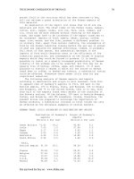
<Table 1> Averages and Standard Deviations of Real GDP Growth Rate
(1971.1Q~2007 2Q)
(Year-on-Year % Change)

Period

1971~1979

1980~1989

1990~1999

2000~2007.2/4

Whole Period

Average

8.1

7.4

6.0

5.0

6.7

Volatility

3.4

3.8

4.8

2.1

3.9

The fast growing Korean economy, dating back to 1960s, has been
showing a sign of gradual slowdown up to present. Especially, the
lowered economic growth after the financial crisis in 1997 is worried to
indicate slowdown in the growth of potential GDP, which attributes at
least partly to the fast aging demographic composition. As seen in
<Table 1>, the average real GDP growth has been falling from marvelous
8.1% during 1970s to 5.0% during 2000s.
In the meantime, the volatility of the GDP growth(measured by
standard deviation) rose from 3.4% during 1970s to 4.8% during 1990s
and fell again to 2.1% during 2000s. Reminded that the East Asian
Currency Crisis broke out in the fourth quarter of 1997, it seems that
the severity of business cycle fluctuations stayed more or less at the same
level up to late 1990s and it was subdued in 2000s (see [Figure 1]). Such
dampening business fluctuation seems to be related with the global
prevalence of low interest rate and the emergence of China as a new
world economic power.
Putting all these into consideration, it would be pivotal to identify

4


post crisis changes in various market institutions of Korea and the global
environments surrounding them for understanding the growth path of
Korean economy (at least) after 1990s. To take a few but most remarkable
post crisis reform measures 2 taken in Korea, an inflation targeting rule
and the floating exchange rate system were introduced, while financial
institutions were restructured.
[Figure 1] Trends of Real GDP Growth Rate (with or without Treatment of Seasonality)
(Year-on-Year % Change, Quarter-on-Quarter % Change)

15

10

5

0

-5

-10
1970

1973

1976

1979

1982

1985

1988

ln(real GDP)

1991

1994

1997

2000

2003

2006

ln(real GDP(S.A))

As is widely believed, financial restructuring led to changes of
behaviors in both demand and supply sides of domestic capital market.
Banks moved their concentration from business finance to consumer
loans in order to reduce risk exposure while enhancing profitability.
Accordingly, households could enjoy the benefit of consumption
smoothing from the alleviation of liquidity constraints (Hur and

Sung[2003]). In the meantime, most large firms, enforced to lower the
debt/equity ratio, began to accommodate required capital by IPOs or
internal reserves rather than by debt financing. By that much, the banks
could hold excess capacity to lend, which in turn directed towards
consumer credit. In addition, the global phenomenon of low interest
rates and mild inflation, which sustained stable growth for the last
Some of these changes were caused by the Crisis but others happened to be taken after (or
around) the outbreak of the Crisis. Here, however, it is not our immediate concern to verify their
causalities with the Crisis. Instead we focus on evaluating the macroeconomic consequences of
these post-crisis changes on the Korean economy.

2

5


decade, contributed to settling the newly adopted inflation targeting rule
(in 1997) and the flexible exchange rate system (in 1998) in post-crisis
Korea.
Admitted that those internal and external environmental changes
may result in lowering the business cycle amplitude, still it remains a
puzzle to explain the slowed pace of economic growth in Korea. Hence,
it would be crucial to devise analytical frameworks beyond merely
introducing major institutional changes so as to include various sources
of shocks and their transmission channels, which may hinder the
economic growth.

2. 2. Literature
In this section we introduce three papers, all of which, in common
with others, explore the economic growth and/or the business cycle of

Korea since 1990s using SVAR. Though, they differ in the time span of
data set used and the pool of variables chosen. Hence, direct comparison
of their results may be not much of consequence. Instead we highlight
their methodological differences.
First, Shim (2001) decomposes post-crisis business cycle by factors
based on B-Q(1989). A linear system of sectoral equations, intended for
deriving long-run restrictions, is arranged so that its Structural Moving
Average Representation (SMAR) or a long-run impulse response matrix
could be formed into a lower or upper triangular one 3. Shim (2001) does
not consider post-crisis changes in the monetary policy rule and the
exchange rate system 4, let alone foreign sectors.
Second, Kim (2005) concentrates on analyzing the impact of foreign
shocks on the domestic business cycle. Hence, Kim uses foreign variables,
such as oil price and exchange rates, jointly with domestic ones
including interest rate, CPI, and the growth rate. Kim (2005)'s model, in
In other words, Shim(2001)'s system of equations is simply reduced to a VAR with Cholesky
ordering.
4 Monetary aggregate targeting and inflation targeting diverge from each other in the treatment
of a money supply schedule. Under the monetary aggregate targeting, LM curve is derived from
money demand=money supply whereas money supply is replaced by an interest rate setting rule,
such as a Taylor rule under the inflation targeting. Furthermore, autonomy of monetary policy
is not guaranteed in a fixed exchange rate system because the domestic interest rate should be
always equal to the foreign interest rate. Otherwise, the exchange rate would fluctuate.
3

6


common with Shim(2001)'s, does not derive the relationship among
shocks from an economic model. Instead he orders them in a Cholesky

way a priori.
Third, Oh (2007) considers an open economy version of the B-Q
model. Matched with three key variables of world import volume, GDP,
and CPI, he introduces three shocks of domestic supply, demand, and
world supply. In terms of shock identification, Oh (2007) also assigns
long-run restrictions to disturbances a priori 5.
Keeping distance from the predecessors, our paper is based on
economic models, which allow the presence of shocks from various
sources and introduces institutional changes in the monetary policy
regime and the foreign exchange market. Then, we derive long-run
restrictions by solving the models and use them in estimating
corresponding SVAR models.

III. Models
In a neoclassical framework, it is somewhat inevitable that an
economy experiences slowdown of growth in the long run. In reality,
however, it is very intricate to distinguish the long-run trend of
slowdown from the short-run business downturns. There are various
statistical methods for decomposing the path of economic growth into
the long run trend and the short-run fluctuations. With the long series of
macro variables available, these statistical methods are relatively easy to
implement but it is not rare to see the results hard to interpret under
conventional economic reasoning.
In contrast, there have been many trials of identifying transmission
channels of shocks with perception that the change of economic growth
is accumulated responses of various sectors to external shocks. Analysis
Oh (2007) assumes that domestic demand shocks have only temporary effect while domestic
supply shocks persist in the long-run. He also assumes that world supply shocks increase
world production and have permanent effect on world demand for imports whereas domestic
supply shocks have only temporary effect on the world demand for imports. Under such

presumptions, the estimation results report that world supply shocks have larger impact in
contrast with the shrunken influence of domestic supply shocks after the financial crisis. It is
also revealed that the impact of domestic demand shocks has been magnified in the short-run.

5

7


in this category, based an economic model (however simple it may be),
allows economic intuition to work but it is not satisfying in that a slight
change in the architecture of the model may lead to a different result. In
this context, additional robustness check would be required.
This study encompasses the first approach from the standpoint of the
second one. In details, it derives long-run restrictions of an SVAR
representation from a simple macro economic model. In the meantime a
number of shocks are introduced in the model. Some of them affect a
sector while others have influence on the economy beyond a sector.
Roughly speaking, those shocks are categorized into two groupsdemand and supply shocks, which are, in turn, believed to match with
business cycle and long-run trend of growth respectively. Behind such a
logic lies a general notion that demand shocks are transient whereas
supply ones are permanent. As admitted by B-Q(1989), however,
transient supply shocks or persistent demand ones may exist in reality.
Thus, it would be absurd to associate demand shocks with volatile
business cycle and supply ones with the changing growth trend. In this
context, our paper keeps itself apart from trials to decompose the
economic growth into the long-run trend and the short run fluctuations

1. Sources of Shocks and Transmission Channels
In the following models all the shocks are classified into demand

driven and supply driven ones, which are, in turn, grouped into
domestic and foreign ones. In addition, we consider the possibility that
the changes of economic environments (internal or external) Korean
economy has experienced since 1990 may have altered transmission
channels while providing new sources of shocks.
To begin with, noticeable internal changes of the economic
environments have been made in restructuring the financial markets and
adopting the inflation targeting rule and the floating exchange rate
system, most of which seem to contribute to altering transmission
channels. On the while, the global phenomenon of low interest rates,
housing price hike and emergence of China as a world economic power
are major external changes surrounding Korean economy.
8


Next, understanding demand and supply shocks within a framework
of AD-AS, we define internal demand shocks to be idiosyncracies in
consumption, investment, government budget, and the markets for
domestic and foreign currencies, and represent external demand shocks
to be rooted in the terms of trade and the world economic growth. On
the other hand, we comprehend that supply shocks are caused internally
by changes in factor and total factor productivities and externally by
price fluctuations of raw materials (such as oil and iron ore) and
technology spill-over.
A notable point here is that such a way of sorting shocks (and
discerning changes in transmission channels from those in the
magnitudes of shocks) is rather conceptual and does not provide a
reliable yardstick to apply in the reality. For example, alleviation of
household credit constraints induced by the restructuring of the financial
sector accompanies consumption growth. Also, it is not fully convincing

to define TFP growth to be a sole domestic supply shock. TFP growth
may results from international competition or TFP growth may interact
with the increased demand for investment. In this regard, our way of
introducing shocks has limitations. As a remedy, we present the four
incomplete models and compare their results instead of searching
indefinitely for just one complete model.

2. Equations of Estimation and Identifying Restrictions
In this study, we estimate the following four SVARs with long run
restrictions. The first two of them, based on Blanchard and Quah(1989),
extend the original version of 2-variables and 2-shocks to a variant of 3variables and 3-shocks, which is to reflect the reality that the Korean
economy is exposed to foreign risks more heavily than other economies.
Thus, we add the inflation ( π t ) to the real GDP growth ( ∆y t ) and the

9


unemployment rate ( U t ) and match them with price shock 6 ( ε tπ ), supply
shock( ε ts ), and demand shock( ε td ) respectively.
The latter two, New Keynesian models borrowed from Stock and
Watson(2002), include the real GDP growth( ∆y t ) and inflation ( π t ) in common.
Then, depending on the types of the monetary policy regime and the

foreign exchange rate system, monetary aggregate growth ( ∆mt ) or
exchange rate change ( ∆et ) is added. In this context, we claim that these
models describes better the real image of Korean economy than B-Q(1989)
type ones 7) .

A. A Three Variable Extension of Blanchard and Quah(1989)
Blanchard and Quah (1989) understand a VAR system in an equivalent

MAR(Moving Average Representation) and levy additional long-run
restrictions on disturbances and their lags 8. B-Q present a simple model
based on Fisher (1979) and provides its solution in the form of long-run
restrictions on demand and supply shocks. Instead of repeating the
already famous B-Q setup, we explain how it is extended to a model with
three variables and three shocks.
As for shocks, we decompose the supply shock into the two parts- the
price shock ( eπt ) and the productivity shock ( ets ) and add them to the
existing demand shock ( etd ). Especially, eπt has direct influence on price
determination, while indirectly working against aggregate demand and
employment .
(1) Aggregate Demand (a combinations of IS and LM urves)
6 Price shocks represent situations like sudden hikes of oil price and foreign exchange rate. By
construction, they denote all the shocks from foreign economies.
7 B-Q(1989) mention that the model in the paper is an example intended for explaining the use of
SVAR with long-run restrictions.
8 SVAR with short run restrictions differs from B-Q(10989) in that it constrains only the
relationships between contemporaneous disturbances.

10


Yt = Mt − Pt + aθ 1 ,t
(2) Aggregate Supply (Assuming a CRS production technology)

Yt = N t + θ 1 ,t
(3) Price Equation

Pt = Wt − θ 1 , t − θ 2 , t
(4) Wage Equation

Wt = W |E

t −1 [ N t

or

]= N

= W |Et −1[U t ] = 0 , U t ≡ N − N t

Et −1[ Wt ] = Wt , Et −1[ N t ] = N

(5) All the shocks of this economy follow AR(1) processes. Furthermore, demand
π

shock( et ), supply shock( et ), and price shock( e t ) are orthogonal to each
s

d

other.

Mt = Mt −1 + etd , θ 1 , t = θ 1 , t −1 + e st , θ 2 , t = θ 2 , t −1 + eπt

Manipulating (1)~(5) properly, we derive the following matrix, in
which key macro variables 9, such as real GDP growth( ∆Yt ), inflation( π t ),
and unemployment rate ( U t ) 10 are represented as moving averages of
exogenous shocks.
1 − 1  e st   − a

∆Yt  ( a + 1)
ed  +  a
 π  =  −1
1
0
t
 t  
 

 U t   − a − 1
1  eπt   0

1  e st −1 


1 − 1  e dt−1 
0
0   eπt −1 

−1

Most of variables are logarized for scaling . In additional all the other variables except the
unemployment rate are used in differences for stationarity.
10
Addition of nominal wage growth ( ∆Wt ) to these three variables, however, would make the
9

SVMAR(Structural Vector Moving Average Representation) under-identified. Hence, we
discard nominal wage growth ( ∆Wt ) from the SVMAR.

11


By simply ignoring the subscripts t and summing the right hand side of the
SVMAR, we obtain the long run restriction matrix C.
1 − 1  − a
( a + 1)
 −1
0
1  +  a

 − a − 1
1   0

−1

1 
1
0 0


1 − 1 = ( a − 1)
1 0
0
0   − a − 1 1

0 
 NA 0

C =  NA NA 0 

 NA NA NA

With these long-run restrictions, all the shocks are exactly identified. Their
effects on the three key variables, both long-run and short-run, are summarized
as follows: To begin with, demand shock( etd ) has temporary effect on the
real GDP whereas it has permanent influence on price level and
unemployment rate. Second, productivity shock ( ets ) affects permanently
all these three macro variables. Third, price shock( eπt ), such as oil price
hike, affects the real GDP and price level temporarily but has permanent
effect on the unemployment rate.

B. An Economy under Inflation Targeting Rule and Flexible Exchange Rate
System

Next, we introduce an open economy New Keynesian model,
substantial part of which is borrowed from Stock and Watson(2002). In
the economy, the government carries out a monetary policy based on
12


inflation targeting 11. In details, it adjusts the short-term interest rate in
response to the anticipated inflation and GDP gap following so called a
Taylor rule.
For the features of openness, we define the trades of commodities,
services and currencies across borders. Hence, we describe an
equilibrium condition for the foreign exchange market and include the
terms of trade 12 ( q t ) as a determinant of IS curve.

(1) IS curve 13
y t = κrt − qt + θ td , θ td ≡ θ td−1 + ε td ,

rt = Rt −

1 k
Et [ π t + j ] , qt = pt − ( et + ptf )
∑
k j =1

(2) New Keynesian Phillips curve(Aggregate supply curve)
∞

π t = γ ∑ δ i Et [ y tp+i − y t +i ] + ε td + ε te
i =0

(3) A forward looking Taylor rule
h

rt = βπ Et [ π t +h ] + β y ∑ δ i Et [ y tp+ j − y t + j ]
j =1

(4) An equilibrium condition in foreign exchange market
Rt = Rtf + Et [ et +1 − et ] + ε te

11 Fiscal policy, another pillar of economic policy, is not considered in the model, which is partly
due to the long-time (at least since mid 1980s) held fiscal stance of so called "expenditure-withinrevenue". In addition, some empirical works report that fiscal stimuli through either increasing
expenditure or reducing tax revenue have not been effective in boosting the Korean economy
(Hur[2007]).
12
Pt
ln Pt
f

qt = p − e − p ⇒ ln Q =
⇒Q =
t t t
t
t
f
f
ln Et Pt
Et Pt
13

IS curve is influenced by the accumulation of demand shocks( ε td ), θ td . It should be noted, however,

that demand shock doesn’t necessarily have permanent effect on yt because yt is determined not only
by the IS curve but also by its interactions with other equilibrium conditions.

13


Equations (1)~(4) consist of orthogonal demand and exchange rate
shock ( ε td , ε te ) and five variables ( yt , Rt , π t , Et [ ytp+i − yt +i ] , et ) 14. Filling the
gap between the numbers of shocks and variables, we define the GDP gap
by an AR(1) process 15 16.
X t ≡ y tp − y t = ρX t −1 + ε ts ,

0 < ρ <1,

(5)

Then, Equation (5) could be represented in moving averages.

X t (1 − ρL ) = ε ts ⇒ X t =

∞
ε ts
= ∑ ρ jε ts− j
1 − ρL j =0

Next, the equilibrium condition of the foreign exchange market is
transformed into Equation (6), which defines the exchange rate ( et ) to be
the sum of interest parity ( Rt − j − Rtf− j ) and the cumulative exchange rate
shock ( θ te ).

et = ( Rt −1 − Rtf−1 ) + et −1 + ε te
= ( Rt −1 − Rtf−1 ) + ( Rt −2 − Rtf−2 ) + et −2 + ε te−1 + ε te
∞

= ∑ ( Rt − j − Rtf− j ) + θ te

(6)

j =1
∞

θ te ≡ ∑ ε te− j
j =0

14

Based on the concenpt of "a small open economy", we assume that interest rate( Rt f ), price

level( ptf ) and inflation ( π t f ) of a foreign country are exogenously given.
15
The author's pretest using the quarterly data of Korea(1979~2001) shows that the GDP

gap( ≡ GDP minus(-) Hodrick-Prescott filtered GDP) follows a stationary AR(1) process ( 0 < ρ < 1 ).
16

With Equations (5) rearranged as ytp = yt + ρX t −1 + ε ts , we could say that this economy is a part

of the Keynesian world in a sense that the potential GDP ( yt p ) moves one-to-one with the
aggregate demand or real GDP ( yt ). However, change in yt will not have any impact on yt + j p (j>0).
Only ε ts will have persistent effect on yt + j p . Once the productivity shock is defined to have
permanent effect on the potential GDP, ε ts in (5) will be a most conceivable candidate for the
productivity shock.

14


Now, we represent the four variables of real GDP( y t ), inflation ( π t ),
nominal interest rate( Rt ), and the exchange rate ( et ) in linear functions
of the three orthogonal shocks ( ε ts , ε td , ε te ).
First, we obtain the following expressions by plugging (5) to the right
hand side of (2) and (3).
∞

π t = χ ∑ δ i Et [ ρXt +i−1 + ε tx+i ] + ε td + ε te
i =0
∞

= χ ∑ δ i ρ i X t + ε td + ε te = χ

i =0

Xt
+ ε td + ε te
1 − δρ

χ ∞ j s
∑ ρ ε t− j + ε td + ε te , (0 ≤ δρ < 1)
1 − δρ j =0

=
=
h

∑ E [y
i =1

t

p
t +i

]

1− ρh
1 − ρ h χρ ∞ j s
Xt =
∑ ρ ε t− j
1− ρ
1 − ρ 1 − δρ j =0

h

− y t +i = ∑ ρ i X t = ρ
i =1

Second, plugging the above equations back to (3), we could represent
the real interest rate ( rt ) as a function of external shocks.
h

rt = βπ Et [ π t +h ] + β y ∑ Et [ y tp+ j − y t + j ]
j =1

 X

1− ρh
Xt
= βπ Et  χ t +h + ε td+h + cε te+h  + β y ρ
1− ρ
 1 − δρ

1− ρh
χρ h
Xt + β y ρ
Xt
= βπ
1 − δρ
1− ρ

χρ h

1− ρh 
X t
=  βπ
+ βy ρ
1 − ρ 
 1 − δρ
Third, converting the expression on the real interest rate ( rt ) to that on
the nominal interest rate ( Rt ) and combining the new expression with (6),
we derive the following.

15


Rt = rt +

[ ]

1 s
∑ Et π t+ j = AXt ,
s j =1

χρ h
1 − ρ h 1 χρ 1 − ρ s
A ≡ βπ
+ βy ρ
+
1 − δρ
1 − ρ s 1 − δρ 1 − ρ
∞

∞

j =1

j =0

et = ∑ ( AXt − j − Rtf− j ) + θ te , θ te ≡ ∑ (φ jε te− j )
Finally, plugging the above equation to (1), we could also represent
the real GDP as a function of external shocks.
y t = κrt − qt + θ td = BX t − qt + θ td ,

1− ρh 
χρ h

B ≡ κ  βπ
+ βy ρ
1 − ρ 
 1 − δρ
Combining all the equations so far derived, we could represent ( yt ,

π t , et ) as moving averages of ( ε ts , ε td , ε te ). As for logarized real GDP( yt )
and the exchange rate ( et ), we use the first order differences for treating
their non-stationarity. Accordingly, the first order differences of the real
GDP( ∆yt ) and the exchange rate ( ∆et ) are represented as follows.
∆y t = B∆X t − qt + qt −1 + θ td − θ td−1
= B∆X t − π t + ( et − et −1 ) + π tf + ε td

χ
X t − ε te + ∆et + π tf ,
1 − δρ

∆X t = (1 − ρL )X t − (1 − ρ )X t −1
= B∆X t −

= ε ts − (1 − ρ )X t −1
∞

= ε ts − ∑ ρ j (1 − ρ )ε ts−1− j
j =0

∆et = et − et −1
∞

∞

∞

j =0

j =0

j =0

= ∑ ( A∆X t − j − ∆Rtf− j ) + ∑ ε te− j − ∑ ε te− j −1

16


Properly rearranged, the vector of ( ∆yt , π t , ∆et ) is represented as a
SVMAR(Structural

Moving

Average

Representation)

exogenous shocks ( ε ts , ε td , ε te ). 17 Furthermore, we could find 3( =

system

of

k × ( k − 1)
, k = 3)
2

∞

restrictions on the coefficients of A∞ ≡ A(1) = ∑ A j . In other words, (7) is exactly identified.
j =0

 ε ts 
 ε ts 
0 
 NA 0
 ∆y t 
 e
 e ∞





 ∆et  = A(L ) ε t  = ∑ A j  ε t  , A∞ =  NA NA 0 
 ε d  j =0  ε d 
 NA NA NA 
π 


 t 
 t 
 t 
The above long-run restriction matrix

A∞ indicates the following

properties of the model economy, which is also characterized by
Equation (1)-(5).

First, the productivity shock ( ε ts ) has permanent

impact on the real GDP, price level, and the exchange rate. Second, the
demand shock ( ε td ) has permanent effect on the price level, but they have
transient effect on the real GDP and the exchange rate. Third, the impact
of the exchange rate shock ( ε te ) has permanent effect on the exchange
rate itself and the price level.

C. An Economy under Monetary Aggregate Targeting Rule and Fixed
Exchange Rate System
The next model differs from the previous one in the selection of the
monetary policy regime as well as the foreign exchange rate system. First,

17

Instead of taking the first order differences of I(1) variables (such as real GDP( yt ) and the

exchange rate of US $ to Korean Won( et )), we could adopt a Structural Vector Error Correction
Model (SVECM) with cointegrating equations, as suggested by King, Plosser, Stock, and
Watson(1991). In contrast, following B-Q(1989), we form a system of SVAR with long-run
identifying restrictions, which consists of I(0) variables and first-order differences of (1)
variables. A reason for not following King et. al.(1989) is to avoid disentangling permanent
shocks from transient shocks apriori.

17


the monetary authority controls a monetary aggregate instead of
adjusting the short-term interest rate based on so called Taylor rule. To
rephrase, it is assumed to closely watch the monetary aggregate (neither
the anticipated inflation rate nor the GDP gap) and use the money
growth (not the short-term interest rate) for a monetary policy tool.
Such a monetary aggregate targeting rule describes best the policy
regime of Bank of Korea before 1997.
Second, the exchange rate is assumed to be fixed at a certain level by
the government. In order to balance the capital account or clear the
currency exchange market at the prespecified exchange rate, interest rate
differential with other countries is not allowed and the monetary
aggregate is constantly controlled for maintaining zero interest rate
differential. In this context, we could say that the central bank loses
autonomy of monetary policy under the fixed exchange rate system. As
in the case of the monetary aggregate targeting, such a fixed or managed
exchange rate system existed until the financial crisis in 1997.

(1) IS curve
y t = κrt − qt + θ tIS , θ tIS = θ tIS−1 + ε tIS ,
rt = Rt −

[ ]

1 k
∑ Et π t+ j , qt = pt − ( et + ptf ) ,
k j =1

π tf ≡ ptf − ptf−1 = S f ,π Xtf
Xtf ≡ y tf ,p − y tf = ρ f Xtf−1
(2) LM curve
mt − pt = yt + bRt
Combining (1) and (2), we derive an aggregate demand schedule as
follows:

κ
yt =

b

(mt − pt ) −

κ
k

(1 +

k

∑ E [π
j =1

t

t+ j

] − qt

aκ
)
b

18

+ θ td , θ td ≡

θ tIS
1+

aκ
b

= θ td−1 + ε td


(3) New Keynesian Phillips curve(Aggregate supply curve) 18
∞

κ
π t = χ ∑ δ i Et [ y tp+i − y t +i ] + (1 + )ε td

b

i =0

(4) An equilibrium condition in foreign exchange market
Rt = Rt f , et = et , Rt f = S f ,R X t f
(5) Money Supply
mt = yt + bRt f + pt

Equation (1)~(4) consist of the demand shock ( ε td ) and four macro
variables ( yt , Rt , π t , mt ). In order to handle with the mismatch, we define
the GDP gap to be an AR(1) process with a noise of ε ts , which is in turn
defined to be the productivity shock.
X t ≡ y tp − y t = ρX t −1 + ε ts , 0 < ρ < 1
X t (1 − ρL ) = ε ts ⇒ X t =

∞
ε ts
= ∑ ρ jε ts− j
1 − ρL j =0

Now, we represent the four variables of the real GDP ( yt ), inflation
( π t ), nominal interest rate ( Rt ), and the monetary aggregate ( mt ) as
functions of the supply shock and the demand shock ( ε ts , ε td ) in the
following procedure. First, inserting the AR(1) representation of the
potential GDP ( X t ) to the right hand side of (3) , we could describe the
inflation ( π t ) to be a function of exogenous shocks.

18

We set demand shock( ε td ) in the New Keynesian aggregate schedule to have a coefficient of
(1 + κ / b ) so that the long-run influence of

ε td on the real GDP could converge to 0.

19


∞
κ
π t = χ ∑ δ i Et [ ρX t −i−1 + ε ts+i ] + (1 + )ε td

b

i =0

κ

∞

= χ ∑ δ i ρ i X t + (1 + )ε td
b
i =0
Xt
κ
=χ
+ (1 + )ε td

b
1 − δρ
=

χ ∞ j s
κ
ρ ε t − j + (1 + )ε td (0 ≤ δρ < 1)
∑
b
1 − δρ j =0

Then, considering the working mechanism of the fixed exchange rate
system, we note that the domestic interest rate ( Rt ) has the following
relationship with the inflation of the foreign economy ( π t f ).

Rt = Rtf = S f ,R X tf , π tf = S f ,π X tf

(7)

Now, we take the first order differences of the real GDP ( yt ) and the
monetary aggregate ( mt ) in consideration of their non-stationarity.

(1 +

κ
κ k
χ
aκ
)∆y t = ( ∆mt − ∆pt ) − ∑
ρ j Xt

b
b
k j =1 1 − ρδ

 χ
κ
− 
X t + (1 + )ε td − S f ,π X tf
b
 1 − ρδ
f
∆mt − ∆pt = ∆y t + b∆Rt


κ
 + (1 + )ε td
b


Then, combining the first order differenced real GDP ( yt ) and
monetary aggregate ( mt ) in the above, we represent the real GDP growth
( ∆y t ) and the money growth ( ∆mt ) to be the moving averages of the
exogenous shocks.

20


∆y t = κ∆Rtf −

κ

χ

k

∑ 1 − ρδ ρ ∆X
k
j =1

j

t

 χ
X t − S f ,π X tf
− 
 1 − ρδ





∆mt = ∆y t + b∆Rtf + π t
∆qt =

χ
κ
χ
κ
X t + (1 + )ε td − π tf =

X t + (1 + )ε td − S f ,π X tf ,
b
b
1 − ρδ
1 − ρδ
∞

∆X t = (1 − ρL )X t − (1 − ρL )X t −1 = ε ts − ∑ ρ j (1 − ρ )ε ts−1− j ,
j =0

Matched with the two shocks ( ε ts , ε td ), ( ∆yt , π t ) are picked out and rearranged
in a SVMAR as below. According to A∞ , the productivity shock ( ε ts ) has
permanent effect on the real GDP only. In contrast, the demand shock
( ε td ) has permanent effect on the price level and the monetary aggregate.

ε s  ∞
ε s 
 ∆y t 
 NA 0 

 = A(L ) td  = ∑ A j  td  , A∞ = 

 πt 
 NA NA 
 ε t  j =0  ε t 
Aforementioned, in the fixed exchange rate system the monetary
authority cannot exercise its discretion in determining the interest rate
and the monetary aggregate. Otherwise, a target exchange rate could not
be maintained. Considering such a dilemma, a bi-variate SVAR with the
real GDP growth and the inflation rate (not with the exchange rate

change) is estimated for the period before the financial crisis.

IV. Estimation Results

1. Data
The data for real GDP, price index (GDP deflator), the exchange rate of
US dollar to Korean won, a monetary aggregate (M2), and the
unemployment rate used in the paper are obtained from the Bank of
Korea. They cover the period between the first quarter of 1970 and the
second quarter of 2007. As a pretest, we examine the existence of unit

21


roots in these variables. Results from DF-GLS procedure (Eliot,
Rothenberg and Stock (1996)) exhibit that all the key variables, such as
the real GDP growth, inflation, the exchange rate change, and the
unemployment rate, do reject the existence of a unit root at 1%
significance level (See <Table 2>).
<Table 2> Unit Root Test Results (DF-GLS)
Test statistic

1% level

5% level

10% level

-2.661

-2.581

-1.943

-1.615

-2.712

-2.581

-1.943

-1.615

-6.068

-2.599

-1.946

-1.614

2.659

-2.581

-1.943

-1.615

(DF-GLS)

∆y t
(GDP deflator)
(

₩K O

Ut

Next, we run various lag-order selection tests. Each of <Table 3> and
<Table 4> reports the test results for B-Q type or New Keynesian type
models. According to them, most of the lag order selection criteria
prescribe longer lags than the data can accommodate. Thus, we take 4
lags in every SVAR estimation 19.
<Table 3> Lag Order Selection Criteria for B-Q type Models
Variables

LR

FPE

AIC

HQIC

SBIC

( ∆y t , U t )

78

33

76

76

76

79

22

38

38

38

( ∆y t ,

π t , Ut )

Notes: 1) The covered period is 1970.1q~2007.2q.
2) LR is likelihood ratio test, FPE is final prediction error, AIC is Akaike's information criterion,
HQIC is Hannan and Quinn information criterion, and SBIC is Schwartz Bayesian information
criterion.

19

A rationale for taking 4 lags is that all the data are gathered on a quarterly basis.

22


<Table 4> Lag Order Selection Criteria for New Keynesian Models

Periods
2000.1/4~2007.2/4
1991.1/4~1997.3/4

Variables
( ∆y t , ∆et

, πt )

( ∆y t , π t )

LR

FPE

AIC

HQIC

SBIC

35

2

60

60

60

48

12

36

36

36

2.. Impulse Responses(IR) and Forecasting Error Variance Decomposition
(FEVD)
We estimate SVAR models based on the long-run restrictions previously
derived. In this section we summarize and analyze the estimation results in
forms of IR and FEVD. IR analysis tracks down the impact of a shock 20 on

an endogenous variable along the passage of time. On the other hand,
FEVD measures the fraction of the error in forecasting the future value of
a variable that is attributable to a shock.

A. Blanchard and Quah(1989)’s original model (2-variables and 2-shocks)

To begin with, we demonstrate the IR and FEVD results for the period
between 1970 Q1 and 2007 Q2 from our benchmark of B-Q(1989)’s
original model. We also estimate the same model for the following four
sub-periods-from 1970 Q1 till 1979 Q4(Period I), from 1980 Q1 till 1989
Q4(Period II), from 1990 Q1 till 1999 Q4(Period III), and from 2000 Q1 till
2007 Q2(Period IV). However, we will mention their results only if
necessary. Such division of the time series is intended to treat structural
changes, which arose from 1970 Q1 till 2007 Q2. 21
IR results in [Figure 2] show that supply shock has permanent effect
on both real GDP and unemployment whereas demand shock affects real
GDP temporarily, which is consistent with the corresponding long-run
The magnitude of a shock is one standard deviation and 95% confidence intervals are calculated by
bootstrappings (1,000 trials each).
21 Instead we could take dummies for certain periods (for example, two oil shocks and the east Asian
financial crisis) and measure the level changes in key macro variables induced by them. But it doesn’t
provide a perfect solution because the dummy variables cannot detect possible functional changes among
the key variables.
20

23


restrictions derived in the previous section. In details, positive supply
shock raises real GDP and temporarily (for the first 20 quarters) lowers
unemployment. In contrast, positive demand shock in the form of money
(M2) growth lowers real GDP although temporarily (for the first 20
quarters) 22.

[Figure 2] Impulse Response of the 2-variable B-Q model
(1970.1/4~2007.2/4)

Real GDP
Supply Shock

Demand Shock

0.030

0.005

0.025

0.000

0.020
-0.005

0.015
-0.010

0.010
-0.015

0.005

-0.020

0.000
0

2

4

6

8

0

10 12 14 16 18 20 22 24

2

4

6

8

10 12 14 16 18 20 22 24

Note: The dotted lines are 95% confidence intervals.

Unemployment rate
Supply Shock

Demand Shock

0.003

0.008

0.002

0.007

0.001

0.006
0.005

0.000

0.004

-0.001

0.003

-0.002

0.002

-0.003

0.001

-0.004

0.000

-0.005

-0.001

-0.006

-0.002
0

2

4

6

8

10 12 14 16 18 20 22 24

0

2

4

6

8

10 12 14 16 18 20 22 24

Note: The dotted lines are 95% confidence intervals.

An observation that unemployment rate rises significantly in response to positive demand shock is
opposite to that of B-Q (1989), which may be attributed to the possibility that in Korea the effect
of demand shock is transmitted faster through price and wage channels. In contrast, in the next
model, which is a three-variable extension of B-Q, such a phenomenon is not sustained
statistically.
22

24


[Figure 3] Forecast Error Variance Decomposition of the 2-variable

B-Q

model (1970.1/4~2007.2/4)
Changes in

Changes in

growth rate of real GDP

unemployment rate
1.0
0.9
0.8

1.00
0.95
0.90

0.7
0.6
0.5
0.4
0.3

0.85
0.80
0.75
0.70

0.2
0.1
0.0

0.65
0.60
1

3

5
7
9
Supply shock

11

13

15
17
19
Demand shock

1

3

5
7
9
Supply shock

11

13 15 17 19
Demand shock

FEVD results in [Figure 3] demonstrates that the relative contribution
of supply shock compared with demand one to the fluctuations of real
GDP growth is roughly 80:20. Conversely, the relative contribution of
demand shock to unemployment rate change is about 85:15.
IR and FEVD results for the previously defined four subperiods are
summarized as follows. First, IR results during Period I, compared with
the whole sample period, show that the magnitude and the persistence of

IRs become smaller and shorter (20 quarters→10 quarters). Furthermore,
FEVD analysis shows that the relative contribution of supply shock to
the movement of real GDP growth is reduced to 60:40 (compare with
80:20 for the whole sample period).
Second, the magnitude of IRs during Period II is close to that during
Period I. However, the persistence of a shock and FEVD results are closer
to those of the whole sample period as in [Figure 2] and [Figure 3].
Third, in comparison with Period I-II, the magnitude of IRs increased
during Period III. Especially, response to supply shock increased
substantially and the persistence of supply shock on the unemployment
rate became longer from 20qaurters to 30 quarters. On the other hand,
the relative contribution of supply shock to the GDP growth rate change
steps back to the level of 1970s(60:40) whereas that of supply shock to
the unemployment fluctuation rises to 70%. We suspect that these
patterns are attributed to the 1997 financial crisis and its aftermath.
25