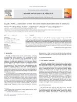
AN0895 oscillator circuits for RTD temperature sensors

AN895
Oscillator Circuits For RTD Temperature Sensors
Author:

RTDs serve as the standard for precision temperature
measurements because of their excellent repeatability
and stability characteristics. A RTD can be characterized over it’s temperature measurement range to
obtain a table of coefficients that can be added to the
measured temperature in order to obtain an accuracy
better than 0.05°C. In addition, RTDs have a very fast
thermal response time.

Ezana Haile and Jim Lepkowski
Microchip Technology Inc.

INTRODUCTION
This application note shows how to design a
temperature sensor oscillator circuit using Microchip’s
low-cost MCP6001 operational amplifier (op amp) and
the MCP6541 comparator. Oscillator circuits can be
used to provide an accurate temperature measurement
with a Resistive Temperature Detector (RTD) sensor.
Oscillators provide a frequency output that is proportional to temperature and are easily integrated into a
microcontroller system.

Two oscillator circuits are shown in Figures 1 and 2 that
can be used with RTDs. The circuit shown in Figure 1
is a state variable RC oscillator that provides an output
frequency that is proportional to the square root of the
product of two temperature-sensing resistors. The
circuit shown in Figure 2, which is referred to as an

astable multi-vibrator or relaxation oscillator, provides a
square wave output with a single comparator. The state
variable oscillator is a good circuit for precision
applications, while the relaxation oscillator is a good
alternative for cost-sensitive applications.

RC oscillators offer several advantages in precision
sensing applications. Oscillators do not require an
Analog-to-Digital Converter (ADC). The accuracy of the
frequency measurement is directly related to the quality
of the microcontroller’s clock signal and high-frequency
oscillators are available with accuracies of better than
10 ppm.
C1

C4

C2

R1 = RTDA

R4

R2 = RTDB
A1

A2

VDD/2

R8

R3

VDD/2

VDD/2

R7
A3
VDD/2

A5

VOUT

VDD

R6

Attributes:

VDD

R5

A4

C5

FIGURE 1:

• Precision dual Element RTD
Sensor Circuit
• Reliable Oscillation Startup
• Freq. ∝ (R1 x R2)1/2

VDD/2

State Variable Oscillator.
R1 = RTD

Attributes:

VDD

C1

A1

VOUT

R2
VDD
R3

FIGURE 2:

R4

•
•
•
•

Low Cost Solution
Single Comparator Circuit
Square Wave Output
Freq. = 1/ (1.386 x R1 x C1)

Relaxation Oscillator.

 2004 Microchip Technology Inc.

DS00895A-page 1


AN895
WHY USE A RTD?

Table 1 provides a comparison of the attributes of
RTDs, thermocouples, thermistors and silicon IC
sensors. RTDs are the standard sensor chosen for
precision sensing applications because of their
excellent repeatability and stability characteristics.
Also, RTDs can be calibrated to an accuracy that is
only limited by the accuracy of the reference
temperature.

RTDs are based on the principle that the resistance of

a metal changes with temperature. RTDs are available
in two basic designs: wire wound and thin film. Wire
wound RTDs are built by winding the sensing wire
around a core to form a coil, while thin film RTDs are
manufactured by depositing a very thin layer of
platinum on a ceramic substrate.

TABLE 1:

ATTRIBUTES OF RTDS, THERMOCOUPLES, THERMISTORS AND SILICON IC
SENSORS

Attribute

RTD

Thermocouple

Thermistor

Silicon IC

Temperature Range

-200 to 850°C

-184 to 1260°C

-55 to +150°C

-55 to +125°C

Temperature (t)
Accuracy

Class B = ±[0.012 +
(0.0019t) -6x10-7t2]

Greater of ±2.2°C
or ±0.75%

Various,
±0.5 to 5°C

Various,
±0.5 to 3°C

Output Signal

≈ 0.00385 Ω/Ω/°C

Voltage (40 µ/°C)

≈ 4% ∆R/∆t for
0°C ≤ t ≤ 70°C

Analog, Serial, Logic,
Duty Cycle

Linerarity

Excellent

Fair

Poor

Good

Precision

Excellent

Fair

Poor

Fair

Good, Power
Specification is
derated with
temperature

Excellent

Durability

Good, Wire wound Good at lower temps.,
prone to open-circuit poor at high temps.,

vibration failures
open-circuit vibration
failures

Thermal Response
Time

Fast (function of
probe material)

Fast (function of
probe material)

Moderate

Slow

Cost

Wire wound - High,
Thin film - Moderate

Low

Low

Moderate

Package Options

Many

Many

Many

Limited, IC packages

Interface Issues

Small ∆R/∆t

Cold junction compensation, Small ∆V

Non-linear resistance

Sensor is located on
PCB

WHY USE AN OSCILLATOR?
There are several different circuit methods available to
accurately measure the resistance of a RTD sensor.
Figure 3 provides simplified block diagrams of three
common RTD-sensing circuits. A constant current,
voltage divider or oscillator circuit can be used to
provide an accurate temperature measurement.
The constant current circuit uses a current source to
create a voltage that is sensed with an ADC. A constant
current circuit offers the advantage that the accuracy of
the amplifier is not affected by the resistance of the

wires that connect to the sensor. This circuit is
especially useful with a small resistance sensor, such
as an RTD with a nominal resistance of 100Ω, where
the resistance of the sensor leads can be significant in
proportion to the sensor’s resistance. In remote
sensing applications, the sensor is connected to the
circuit via a long wire and multiple connectors. Thus,
the connection resistance can be significant. The
resistance of 18 gauge copper wire is 6.5 mΩ/ft. at
25°C. Therefore, the wire resistance can typically be
neglected in most applications.

DS00895A-page 2

The constant current approach is often used in
laboratory-grade precision equipment with a 4-lead
RTD. The 4-lead RTD circuits can be used to provide a
Kelvin resistance measurement that nulls out the
resistance of the sensor leads. Kelvin circuits are
relatively complex and are typically used in only very
precise applications that require a measurement
accuracy of better than 0.1°C.
Another advantage of the constant current approach is
that the voltage output is linear. While linearity is
important in analog systems, it is not usually a critical
parameter in a digital system. A table look-up method
that provides linear interpolation of temperature steps
of 5°C is adequate for most applications and can be
easily implemented with a microcontroller.
The voltage divider circuit uses a constant voltage to

create a voltage that is proportional to the RTD’s
resistance. This method is simple to implement and
also offers the advantage that precision IC voltage
references are readily available. The main
disadvantage of both the voltage divider and constant
current approach is that an ADC is required. The

 2004 Microchip Technology Inc.


AN895
accuracy of the voltage-to-temperature conversion is
limited by the resolution of the ADC and the noise level
on the PCB.
Oscillators offer several advantages over the constant
current and voltage RTD sensing circuits. The main
advantage of the oscillator is that an ADC is not
required. Another key attribute of oscillators is that
these circuits can produce an accuracy and resolution
that is much better than an analog output voltage
circuit. The accuracy of the frequency-to-temperature
conversion is limited only by the accuracy of the
counter or microcontroller time processing unit’s high

Designers are often reluctant to use oscillators due to
their lack of familiarity with these circuits. A negative
feature with oscillators is that they can be difficult to
troubleshoot and may not oscillate under all conditions.
However, the state variable and relaxation oscillators
provide very robust start-up oscillation characteristics.

Clock

Precision
Constant Current Circuit
Current
Source

IREF

frequency clock signal. High frequency clock signals
are available with an accuracy better than 10 ppm over
an operating temperature range of -40°C to +125°C. In
addition, the temperature sensitivity of the reference
clock signal can usually be compensated with a simple
calibration procedure.

Attributes:
VOUT

Amplifier

®

Anti-Aliasing
Filter

ADC

• Insensitive to resistance of

leads with Kelvin connection
• Temperature proportional to
resistance (Temp. ∝ RRTD)
• Constant current source
circuits typically require a VREF
and several op amps

PICmicro
Microcontroller

RRTD
VOUT = IREF x RRTD

VREF

Clock

Voltage Divider Circuit

Attributes:

R
VOUT

Amplifier

Anti-Aliasing
Filter

ADC

PICmicro®
Microcontroller

• Most popular method
• Temperature proportional to
resistance (Temp. ∝ 1 / RRTD)
• Precision VREF ICs are readily
available

RRTD
VOUT = [RRTD / (R +RRTD)] x VREF

RC Oscillator

Clock

RRTD

Attributes:
PICmicro®
Microcontroller

RC Oscillator
freq.∝ RRTD

FIGURE 3:

• Does not require ADC or VREF
• Excellent noise immunity

• Accuracy proportional to quality
of microcontroller clock

Common RTD Sensor Signal Conditioning Circuits.

 2004 Microchip Technology Inc.

DS00895A-page 3


AN895
STATE VARIABLE OSCILLATOR
Circuit Description
The schematic of the circuit is shown in Figure 1. The
state variable oscillator consists of two integrators and
an inverter. Each integrator provides a phase shift of
90°, while the inverter adds an additional 180° phase
shift. The total phase shift of the three amplifiers is
equal to 360°, with an oscillation produced when the
output of the third amplifier is connected to the first
amplifier.
The first integrator stage consists of amplifier A1, RTD
resistor R1 (RTDA) and capacitor C1. The second
integrator consists of amplifier A2, RTD resistor R2
(RTDB) and capacitor C2. For a dual RTD sensing
application, R1 ≅ R2 and C1 and C2 should be the same
value. The inverter stage consists of amplifier A3,
resistors R3 and R4 and capacitor C4. The addition of
capacitor C4 helps ensure oscillation start-up.
A dual-element RTD is used to increase the difference

in the oscillation frequency from the minimum to the
maximum sensed temperature. The state variable
oscillator’s frequency is proportional to the square root
of the product of the two RTD resistors
(frequency ∝ (R1 x R2)1/2). In contrast, a singleelement RTD will produce a frequency output that is
proportional to the square root of the RTD
(frequency ∝ (R1)1/2). If the RTD resistance changes
by a factor of two over the temperature sensing range,
a dual-element sensor will provide an output that
doubles in frequency. A single-element RTD will
produce an output that varies by only 41% (i.e., √2).
The state variable circuit offers the advantage that a
limit circuit is not required if rail-to-rail input/output
(RRIO) amplifiers are used and the gain of the inverter
stage A3 is equal to one (i.e., R3 = R4). In contrast, most
oscillators require a limit or clamping circuit to prevent
the amplifiers from saturating. The gain of the
integrator stages A1 and A2 is equal to one at the
oscillation frequency, as shown by the detailed design
equations provided in Appendix B: “Derivation of
Oscillation Equations”.
Amplifier A4 is used the provide the mid-supply
reference voltage (VDD/2) required for the singlesupply voltage circuit. Resistors R5 and R6 form a voltage divider, while capacitor C5 is used to provide noise
filtering.

Design Procedure
A simplified design procedure for selecting the resistors and capacitors is provided below. A detailed derivation of the equations is provided in Appendix B:
“Derivation of Oscillation Equations”.
The state variable oscillator design equations can be
simplified by selecting identical integrator stages (A1

and A2) and by using an inverter (A3 with a gain of one).
The identical integrator stages are implemented by
using a dual-element RTD sensor and selecting C1= C2.
A unity-gain inverter stage is achieved if R3 = R4.
Simplified Equations:
Assume:
1.
2.
3.

R1 = R2 = R (RTDA = RTDB)
C1 = C2 = C
R3 = R4

Design Procedure:
1.

2.

Select a desired nominal oscillation frequency
for the RTD oscillator. Guidelines for selecting
the oscillation frequency are provided in the
“System Integration” section of this
document.
C = 1/(2πRofo).

3.

Select an op amp with a GBWP ≥ 100 x fmax.

where:

Ro = RTD resistance at 0°C

where: fmax = 1 / (2πRminC) and Rmin = RTD
resistance at coldest sensing temperature.
4.
5.

Select R3 = R4 equal to 1 to 10 times Ro.
Select C4 using the following equations:
f-3dB = 1 / (2πR4C4)
C4 ≈ 1 / (2πR4f-3dB)
where: f-3dB ≅ op amp’s GBWP

Listed below is the hysteresis equation for comparator
A5. The comparator functions as a zero-crossing
detector that is offset by the voltage VDD/2.
R7
V HYS = ------------------- × ( VOUT ( max ) – V OUT ( min ) )
R 7 + R8
R7
VHYS ≅ ------ × VDD
if R8 >>R7
R
8

Comparator A5 is used to convert the sinewave output
to a square wave digital signal. The comparator
functions as a zero-crossing detector and the switching

point is equal to the mid-supply voltage (i.e., VDD/2).
Resistor R8 is used to provide additional hysteresis
(VHYS) to the comparator.

DS00895A-page 4

 2004 Microchip Technology Inc.


AN895
State Variable Test Results

TABLE 2:

The components used in the evaluation design are
listed in Table 2. The circuit was tested with lab stock
components. The specifications of the 100 nF
capacitors are not as good as the NPO porcelain
ceramic capacitors used in the RSS error analysis
shown in Table 4. The maximum capacitance available
with the ATC700 series NPO capacitors is 5100 pF.
The decrease in magnitude of C1 and C2 will increase
the oscillation frequency from 21 kHz to 39 kHz for a
RTD sensed temperature of -55°C to +125°C. If smaller
magnitude capacitors are used, a MCP6024 op amp
with a GBWP of 10 MHz is recommended to minimize
the op amp error on the accuracy of the higher
oscillation frequency.

R1, R2 = Dual Platinum Thin-Film

RTD Temperature Sensor
Omega 2PT1000FR1345
RO = 1000Ω
Accuracy = Class B
R3, R4, R5, R6, R7 = 1 kΩ
R8 = 1 MΩ
C1,C2 = 100 nF
C4 = 20 pF
C5 = 1 µF
VDD = 5.0V
VSS = Ground

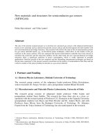
The test results are shown in Table 3 and Figure 4. The
oscillation frequency was calculated using the
measured values of R1, R2, R3, R4, C1 and C2. The
dual-element RTD sensors (R1 and R2) were tested by
simulating a change in temperature with discrete
resistors and measuring the resistance to a resolution
of 100 mΩ. Capacitors C1 and C2 were measured to
have a capacitance of 100.4 nF and 100.8 nF,
respectively.

TABLE 3:

STATE VARIABLE
COMPONENTS

A1, A2, A3, A4 = MCP6004 op amp
(quad RRIO,
GBWP = 1 MHZ)

A5 = MCP6541 Push-Pull
Output Comparator

STATE VARIABLE OSCILLATOR TEST RESULTS

Simulated
Temperature (°C)

Resistor Values
(R1 = R2 =)(Ω)

Calculated Frequency
(Hz)

Measured Frequency
(Hz)

Error
(%)

Error
(°C)

-50.4

806

1961

1957

+0.20

0.52

-20.8

920

1718

1715

+0.16

0.42

0

1000

1581

1577

+0.24

0.62

26.0

1100

1440

1443

-0.23

0.60

51.9

1200

1317

1321

-0.29

0.75

75.3

1290

1225

1223

+0.24

0.62

98.7

1380

1146

1144

+0.20

0.52

122.1

1470

1076

1073

+0.25

0.65

s

Output of Amplifier A3 (V3)

Comparator Output A5 (VOUT)

FIGURE 4:

State Variable Oscillator Test Results (R1 = R2 = 1000Ω ).

 2004 Microchip Technology Inc.

DS00895A-page 5


AN895
Error Analysis
Error analysis is useful to predict the manufacturing
variability, temperature stability and the drift in accuracy
over time. The majority of the error, or uncertainty in the
state variable oscillation frequency, results from the
resistors and capacitors. The errors caused by the PCB
layout and op amp are small in comparison. The
frequency errors that result from the PCB layout can be
minimized by using good analog PCB layout techniques. The error of the amplifier is minimized by
selecting an op amp with a GBWP of approximately
100 times larger than the oscillator frequency.
Table 4 provides a Root Sum Squared (RSS)
estimation of the resistor and capacitor errors on the
frequency output of the state variable oscillator. Note
that capacitor C4 is not included in the table because it

will not be a factor in the oscillation equation, if it’s
magnitude is relatively small. The equation that
specifies the accuracy of a class B RTD is given in
Appendix A: “RTD Selection”. The RTD has a
temperature accuracy of ±0.15°C at room temperature
and ±0.35°C at +125°C. Together, the state variable
oscillator and a class B dual-element RTD will provide
a
temperature
measurement
accuracy
of
approximately ±0.67°C at room temperature and
±1.07°C at +125°C.

TABLE 4:

Temperature compensation can be used to improve the
accuracy of the circuit. The component tolerance error
term of resistors R3 and R4, capacitors C1 and C2 and
the RTD resistors R1 and R2 can be minimized by
calibrating the oscillator to a single known temperature.
The magnitude of the resistor and capacitor
temperature coefficient terms can be minimized by
selecting low temperature coefficient components and
by calibrating the circuit at multiple temperatures.
Resistors with small temperature coefficients are
readily available. However, the temperature coefficient
of a capacitor is relatively large in comparison. A
constant change in the capacitance can easily be

compensated, though the temperature coefficient of a
capacitor is usually not linear. The temperature
coefficient of most capacitors is small at +25°C and
much larger at the extreme cold and hot ends of the
temperature range.
The aging or long-term stability error of the circuit is
minimized by selecting components with a small drift
rate. This term can also be reduced by using a burn-in
procedure. Temperature compensation and burn-in
options are discussed in the “Oscillator Component
Selection Guidelines” section of this document. The
state variable circuit and a class B RTD can be used to
provide a measurement accuracy better than ±0.1°C
with temperature compensation and a burn-in
procedure.

ERROR ANALYSIS OF RESISTORS, CAPACITORS AND RTD ON OUTPUT OF STATE
VARIABLE OSCILLATOR (NOTE 4)
Item

Sensitivity
(Notes 1,
2 and 5)

Error @ +25°C

Error @ +125°C

R3, R4

-0.5, +0.5

100 ppm

100 ppm

Tolerance = 0.01%
RNC90

Resistor TC

R3, R4

-0.5, +0.5

0 ppm

200 ppm

TC = 2 ppm/°C

Resistor Aging

R3, R4

-0.5, +0.5

50 ppm

50 ppm

∆R at 2000 hours,
0.3W and +125°C

Capacitor Tolerance

C1, C2

-0.5, -0.5

2500 ppm

2500 ppm

Tolerance = 0.25%
NPO Porcelain Ceramic
(ATC700B series,
American Technical
Ceramic)

Capacitor TC

C1, C2

-0.5, -0.5

0 ppm

3000 ppm

TC = 30 ppm/°C

Capacitor Aging

C1, C2

-0.5, -0.5

0 ppm
(zero aging effect)

0 ppm
(zero aging effect)

Capacitor Retrace

C1, C2

-0.5, -0.5

200 ppm

200 ppm

∆C temperature hysteresis

RTD Accuracy

R1, R2

-0.5, -0.5

643 ppm

1340 ppm

Class B dual element RTD

Error Term
Resistor Tolerance

Note 1:
2:
3:
4:
5:

Comments

∆C at 2000 hours, 200%
WVDC and +125°C

The sensitivity of the resistors is defined as the relative change in the oscillation frequency per the relative
change in resistance ((∆fo/fo)/(∆R/R)).
The sensitivity of the capacitors is defined as the relative change in the oscillation frequency per the
relative change in capacitance ((∆fo/fo)/(∆C/C)).
The temperature accuracy error (∆t) was calculated using the equations provided in Table 7.
ppm is defined as parts-per-million (i.e., 200 ppm = 0.02%).
The sensitivity equations are defined in Appendix C: “Error Analysis”.

DS00895A-page 6

 2004 Microchip Technology Inc.


AN895
TABLE 4:

ERROR ANALYSIS OF RESISTORS, CAPACITORS AND RTD ON OUTPUT OF STATE
VARIABLE OSCILLATOR (NOTE 4) (CON’T)

Error Term

Item

Sensitivity
(Notes 1,
2 and 5)

Error @ +25°C

Error @ +125°C

∆freq. (∆f)

3493 ppm / 0.349%

7390 ppm / 0.739%

∆temp. (∆t)

∆t = ±0.91°C

∆t = ±1.93°C

Worst-Case Error

Note 3

RSS Error

Note 3

∆freq. (∆f)

2592 ppm / 0.259%

4140 ppm / 0.414%

∆temp. (∆t)

∆t = ±0.67°C

∆t = ±1.07°C

Note 1:
2:
3:
4:
5:

Comments

The sensitivity of the resistors is defined as the relative change in the oscillation frequency per the relative
change in resistance ((∆fo/fo)/(∆R/R)).
The sensitivity of the capacitors is defined as the relative change in the oscillation frequency per the
relative change in capacitance ((∆fo/fo)/(∆C/C)).
The temperature accuracy error (∆t) was calculated using the equations provided in Table 7.
ppm is defined as parts-per-million (i.e., 200 ppm = 0.02%).
The sensitivity equations are defined in Appendix C: “Error Analysis”.

 2004 Microchip Technology Inc.

DS00895A-page 7


AN895
RELAXATION OSCILLATOR
Circuit Description
The relaxation oscillator shown in Figure 5 provides a
resistive sensor oscillator circuit using the MCP6541
comparator. This circuit provides a relatively simple
and inexpensive solution to interface a resistive sensor,
such as a RTD to a microcontroller. This circuit
topology requires a single comparator, a capacitor and
a few resistors. The oscillator outputs a square wave
with a frequency proportional to the change in the
sensor resistance.
The analysis of this circuit begins by assuming that
during power-up, the comparator output voltage is

railed to the positive supply voltage (VDD). Based on
the values of R2, R3 and R4, the voltage at VIN+ of the
comparator can be determined. This voltage becomes
a switching or trip voltage to toggle the output to VSS as
the voltage across the capacitor C1 charges.
The comparator sources current to charge the
capacitor through the feedback resistor (R1). When the
voltage across the capacitor rises above the voltage at
VIN+, the comparator drives the output down to the
negative rail (VSS). However, when the output voltage
swings to VSS, the trip voltage at VIN+ also changes.
Now the comparator output stays at VSS until the
voltage across the capacitor discharges through R1.
When the capacitor voltage falls below the voltage at
VIN+, the comparator drives the output up to the positive rail (VDD). Therefore, the comparator swings the
output voltage to the rails (VDD and VSS), every time the
capacitor voltage passes the trip voltage. As a result,
the comparator output generates a square wave
oscillation.

Simplified Equations:
Assume:
1.
2.
3.

R1 = RTD sensor
R2 = R3 = R4 = R
R ≅ 10 x Ro
where:

Ro = RTD resistance at 0°C

Design Procedure:
1.

2.
3.

Select a desired nominal oscillation frequency
for the RTD oscillator. Guidelines for selecting
the oscillation frequency are provided in the
“System Integration” of this document.
C1 = 1 / (1.386 Ro fo).
Select a comparator with an Output Short
Circuit Current (ISC) which is at least five times
greater than the maximum output current to
ensure start-up at cold and relatively good
accuracy.
IOUT_MAX = VDD / R1_MIN
ISC = IOUT_MAX / 5
where: R1_MIN = RTD resistance at coldest
sensing temperature and VDD is equal to the
supply voltage.

Relaxation Oscillator Test Results
The oscillation frequency was calculated using fixed
discrete resistors to simulate the RTD resistance, R1
and the component values shown in Figure 5. A
0.68 µF tantalum capacitor was chosen for C1. The

circuit uses the MCP6541 comparator.
R1 = RTD
(1 kΩ @ 0°C)

Design Procedure
A simplified design procedure for selecting the resistors
and capacitor C1 is provided below. The relaxation
oscillator design equations can be simplified by selecting the trip point voltages of the comparator circuit to be
equal to 1/3 VDD and 2/3 VDD by using equal value
resistors for R2, R3 and R4. A detailed derivation of the
oscillation equations and error terms is provided in
Appendix B: “Derivation of Oscillation Equations”.

C1
VDD

0.68 µF
VIN-

MCP6541

VOUT

VIN+
VDD

R2
10 kΩ

R4

R3 10 kΩ
10 kΩ

FIGURE 5:
Relaxation Oscillator
Component Values.

DS00895A-page 8

 2004 Microchip Technology Inc.


AN895
TABLE 5:

RELAXATION OSCILLATOR TEST RESULTS

Simulated Temperature
(°C)

RTD
(Ω)

Calculated Frequency
(Hz)

Measured Frequency
(Hz)

Error

(%)

Error
(°C)

-51.7

801

1322.4

1303

-1.47

3.9

-18.2

930

1139.0

1124

-1.31

3.5

12.5

1048

1010.7

1000

-1.06

2.8

25.5

1098

964.7

955

-1.01

2.7

54.0

1208

876.9

867

-1.12

2.9

76.4

1294

818.6

811

-0.93

2.4

95.3

1367

774.9

769

-0.76

2.0

120.8

1465

723.0

717

-0.83

2.2

Table 5 shows a summary of the test results, while
Figure 6 provides a picture of the oscillation frequency
from the oscilloscope.

configurations. The growing popularity of the thin film
technology has resulted in larger resistance RTDs at a
reasonable cost.
Another factor that limits the accuracy of the relaxation
oscillator is the relatively poor performance
characteristics of the 0.68 µF capacitor. Recommendations on the selection of capacitor C1 to maximize the
accuracy of the oscillation frequency are provided in
the section titled, “Oscillator Component Selection
Guidelines”.

Error Analysis

FIGURE 6:
Oscillator Output.

Measured Relaxation

A major error source in the relaxation oscillator is the
comparator’s output drive capability. When the output
of the comparator toggles to VDD or VSS, the
comparator has to source and sink the charge and
discharge current. If the comparator output is current
limited, it takes a longer period of time to charge and
discharge the capacitor C1, which ultimately affects the
oscillation frequency. The oscillation frequency needs
to be properly selected so that the comparator’s output
limits introduce a relatively small error over the oscillation frequency range. This error source is described in
Appendix D: “Error Analysis of the Relaxation
Oscillator’s Comparator”.
If a larger resistance RTD sensor is used, the
comparator’s output current is reduced and the
accuracy of the circuit increases. RTD sensors are
available in a number of nominal resistances, including
2000Ω and 5000Ω. The test results of Table 5 show
that the relaxation oscillator’s accuracy is greater at the
larger resistances than at the smaller resistances. The
1000Ω RTD resistance was chosen because it is
readily available in both wire wound and thin film

 2004 Microchip Technology Inc.

Table 6 provides a RSS estimation of the error of the
resistors and capacitor on the output frequency of the
relaxation oscillator. The test results from the previous
section show that the comparator output drive

capability limits the circuit accuracy. To minimize this
affect, a smaller capacitor and larger RTD resistance
can be used (see Appendix D: “Error Analysis of the
Relaxation Oscillator’s Comparator”).
The sensitivity equations for the relaxation oscillator
are listed below. The sensitivity values of resistors R3
and R4 will be determined from the design equations
provided in Appendix B: “Derivation of Oscillation
Equations”. Note that R2 does not have a sensitivity
term because a change in the resistance changes the
upper and lower trip voltages an equal amount at the
inverting terminal and the voltage level difference
between the trip voltages will remain constant.
Although resistor R2 does not play a critical role in
determining the oscillation frequency, it is
recommended that the circuit use a high-quality
resistor equal to R3 and R4.
1
f o = -----------------------------------( 1.386 ) ( R1 C1 )
fo

fo

1

1

SR = SC = – 1

fo

fo

3

4

S R = – S R = – 0.716

The RSS analysis shows that the resistors, capacitors
and RTD errors limit the accuracy of the oscillator to
approximately 1.2% at room temperature and 1.5% at
+125°C, which corresponds to a temperature

DS00895A-page 9


AN895
resolution of ±3.3°C and ±3.9°C, respectively. The
equations correlating the oscillator’s frequency to the
temperature are provided in the “System Integration”
section of this document.

accuracy of the circuit are discussed in the “Oscillator
Component Selection Guidelines” section of this
document.

The major error term of the relaxation oscillator is due
to the tolerance of the capacitor. Thus, a calibration of
the capacitor’s nominal value can improve the

accuracy of the temperature measurement. Options for
providing temperature compensation to improve the

TABLE 6:

ERROR ANALYSIS OF RELAXATION RESISTORS, CAPACITORS AND RTD (NOTE 4)

Error Term

Item

Sensitivity
(Notes 1,
2 and 5)

Error @ +25°C

Error @ +125°C

Comments

Resistor Tolerance

R3, R4

-0.716,
+0.716

1000 ppm

1000 ppm

Tolerance = 0.1%,
RN55 metal film

Resistor TC

R3, R4

-0.716,
+0.716

0 ppm

5000 ppm

TC = 50 ppm/°C

Resistor Aging

R3, R4

-0.716,
+0.716

5000 ppm

5000 ppm

∆R at 2000 hours, 0.3W

and +125°C

Capacitor Tolerance

C1

-1

10000 ppm

10000 ppm

Tolerance = 1%,
NPO multi-layer ceramic
(Presidio Components Inc. ®)

Capacitor TC

C1

-1

0 ppm

3000 ppm

TC = 30 ppm/°C

Capacitor Aging

C1

-1

0 ppm
(zero aging effect)

Capacitor Retrace

C1

-1

200 ppm

200 ppm

∆C temperature hysteresis

RTD Accuracy

R1,

-1

643 ppm

1340 ppm

Class B RTD

0 ppm
∆C at 2000 hours, 200%
(zero aging effect) WVDC and +125°C

Worst-Case Error

Note 3

∆freq. (∆f)

19435 ppm/1.94%

30292 ppm/3.03%

∆temp. (∆t)

∆t = ±5.2°C

∆t = ±8.1°C

∆freq. (∆f)

12400 ppm/1.24%

14677 ppm/1.47%

∆temp. (∆t)

∆t = ±3.3°C

∆t = ±3.9°C

RSS Error

Note 1:
2:
3:
4:
5:

Note 3

The sensitivity of the resistors is defined as the relative change in the oscillation frequency per the relative
change in resistance ((∆fo/fo)/(∆R/R)).
The sensitivity of the capacitors is defined as the relative change in the oscillation frequency per the
relative change in capacitance ((∆fo/fo)/(∆C/C)).
The temperature accuracy error (∆t) was calculated using the equations provided in Table 7.
ppm is defined as parts-per-million (i.e., 200 ppm = 0.02%).
The sensitivity equations are defined in Appendix C: “Error Analysis”.

DS00895A-page 10

 2004 Microchip Technology Inc.


AN895
OSCILLATOR COMPONENT
SELECTION GUIDELINES
Calibration and Burn-In

An oscillator used in sensor applications must have a
tight tolerance, a small temperature coefficient and a
low drift rate. The op amps, resistors and capacitors
must be chosen carefully so that the change in the
oscillation frequency results primarily from the change
in the resistance of the RTD sensor and not from
changes in the values of the other components.
An application that requires an oscillator accuracy of
better than approximately ±1°C may require a
temperature calibration and/or burn-in procedure to
achieve the desired accuracy. A temperature
compensation algorithm can be easily implemented
using the EEPROM non-volatile memory of a
PICmicro® microcontroller to store temperature correction data in a look-up table. The temperature coefficients are obtained by calibrating the circuit over the
operating temperature range and comparing the measured temperature against the actual temperature. A
polynomial curve-fitting equation of the frequency
versus temperature data can also be used to improve
the accuracy of the oscillator. Since the compensation
coefficients will be unique for each PCB, the cost of
manufacturing will increase.
The drift error of the resistors and capacitors can be
significantly reduced by using a burn-in or temperaturecycling procedure. The long-term stability of resistors
and capacitors is typically specified by a life test of
2000 hours at the maximum rated power and ambient
temperature. Burn-in procedures are successful in
stabilizing the drift error because the majority of the
change in magnitude of resistors and capacitors
typically occurs in the first 500 hours and the
component drift is relatively small for the remainder of
the test. A temperature-cycling procedure that exposes

the components to fast temperature transients from
cold-to-hot and hot-to-cold can be used to reduce the
mechanical stresses inherent in the devices and
improve the long-term stability of the oscillator.

Op Amp Selection
The appropriate op amp to use for the state variable
oscillator can be determined with a couple of general
design guides. First, the Gain Bandwidth Product
(GBWP) should be a factor of approximately 100 times
higher than the maximum oscillation frequency. Next,
the Full Power Bandwidth (fP) should be at least 2 times
greater than the maximum oscillation frequency. The
MCP6001 amplifier has a GBWP = 1 MHz (typ.) and a
fP of approximately 30 kHz, with VDD = 5V. An oscillator
with a frequency of approximately 10 kHz can be
implemented with the MCP6001 with enough design
margin that the op amp errors can be neglected.

 2004 Microchip Technology Inc.

Comparator Selection
The accuracy of the relaxation oscillator can be
improved by using a comparator rather than an op amp
for the amplifier. A comparator offers several
advantages over an op amp in a non-linear switching
circuit, such as a square wave oscillator. An op amp is
intended to operate as a linear amplifier, while the
comparator is designed to function as a fast switch.
The switching specifications, such as propagation

delay and rise/fall time of a comparator, are typically
much better than an op amp’s specifications. Also, the
switching characteristics of an op amp typically only
consist of a slew rate specification.
The non-ideal characteristics of a comparator will
produce an error in the expected oscillation frequency.
The offset voltage (VOS), input bias current (IB),
propagation delay, rise/fall time and output current limit
have an effect on the oscillation frequency. The nonideal characteristics of the MCP6541 comparator are
analyzed in Appendix D: “Error Analysis of the
Relaxation Oscillator’s Comparator” and the resulting frequency error of the relaxation oscillation is
estimated. The test results of the relaxation oscillator
show that an accuracy of approximately ±3°C can be
achieved using the MCP6541 using a 1000Ω RTD. The
accuracy of the relaxation oscillator can be improved
by using a higher-resistance RTD and a higher
performance comparator. However, the trade-off will be
that the comparator’s current consumption will be much
higher.

Resistor Selection
The errors of the resistors can be minimized by
selecting precision components and will be much less
than the error from the capacitors. Metal film and foil
resistors are two types of precision resistors that can
be used in an oscillator. Metal film resistors are
available with a tolerance of 0.01%, TC of ±10 to
±25 ppm/°C and a drift specification of approximately
0.1 to 0.5%. RNC90 metal foil resistors are available
with a tolerance of 0.01%, temperature coefficient of

±2 ppm/°C and a drift specification of less than 50 ppm.
Vendors, such as Vishay® Intertechnology, Inc., offer a
number of precision resistors that have much better
specifications than the RNC90. These devices,
however, are relatively expensive.
The operating environment of a resistor also can
induce a change in resistance. Though the change of
the ambient temperature is usually unavoidable; however, the power rating of a resistor can be chosen to
minimize any self-heating from the I2R drop of the
device. Other factors, such as humidity, voltage coefficient (∆R versus voltage) and thermal EMF (due to the
temperature difference between the leads and selfheating) are small and can be neglected by using
quality components and standard low noise analog
PCB layout procedures.

DS00895A-page 11


AN895
Capacitor Selection
Capacitors have relatively poor performance when
compared with resistors and are usually the component
that limits the accuracy of an oscillator. Furthermore,
precision capacitors are available in only relatively
small capacitances. The state variable circuit reference
design requires two 100 nF capacitors, while the relaxation oscillator needs a 0.68 µF capacitor in order for
both circuits to have a nominal frequency of approximately 1 kHz, with a 1 kHz RTD. A capacitor with a tight
tolerance, low temperature coefficient and small drift
rate is available only in a maximum capacitance of
approximately 100 nF. The relatively poor specifications of a microfarad-range capacitor limits the
accuracy of the relaxation oscillator to approximately

3°C, unless temperature compensation is provided.
The major environmental error term of a capacitor is
due to temperature hysteresis and is specified as the
retrace error. Precision sensors can use temperature
compensation to correct for a change of capacitance
with temperature. However, it is difficult to correct for
hysteresis errors. The retrace error of the American
Technical Ceramic’s ATC700 capacitors recommended
for the state variable oscillator is specified at ± 0.02%.
Other capacitor environmental errors result from the
piezoelectric effect (∆C versus voltage and pressure),
the quality factor (Q) and resistance of the terminals.
These errors are relatively small and can be neglected.
In a sensor application, the oscillation frequency is well
below the capacitor’s maximum rated frequency and
the amplitude of the voltage is small compared to the
maximum Working Voltage DC (WVDC) rating of the
capacitor.
RF and microwave capacitors are a good source of
precision capacitors for the state variable oscillator.
The ATC700 series NPO porcelain and ceramic
capacitors have a tolerance of 0.1 pF, a temperature
coefficient of 0 ±30 ppm/°C and a drift rating of 0.00%.
Note that the vendor’s data sheet states that the NPO
dielectric has no change in capacitance with aging.
However, the military standard for the device specifies
the aging error as less than 0.02%. The trade-off with
the high-frequency ATC700 NPO capacitors is that
they are relatively small in magnitude and are only
available in a maximum capacitance of 5100 pF.

a drift rating of 0.5%. One additional problem with the
polypropylene capacitors is that their maximum
temperature is typically specified at +85 to +105°C and
some of the devices will not withstand the heat of an
automated PCB soldering system.

SYSTEM INTEGRATION
Oscillator to PICmicro® Microcontroller
Interface
The op amp oscillator can be easily integrated with a
PICmicro microcontroller to determine the frequency of
the oscillation or temperature. The oscillator can be
connected to the PICmicro microcontroller with a
standard digital input pin. However, a Schmitt-triggered
input is recommended to provide additional noise
immunity. A critical component in the frequency
measurement system is the microcontroller’s clock
signal. The accuracy of the frequency measurement is
directly related to the accuracy of the clock signal.
Clock
RRTD

RC
Oscillator

PICmicro®
Microcontroller

FIGURE 7:

Typical RC Op Amp
Oscillator Sensor System.

A multi-layer or stacked NPO ceramic is the
recommended capacitor for the relaxation oscillator.
Vendors (such as Presidio, etc.) offer multi-layer NPO
capacitors in values that include microfarads. Multilayer capacitors are available with a tolerance of 1%, a
temperature coefficient of 0 ±30 ppm/°C and a zero
drift rating. Other types of capacitors available in a
range of approximately 1 µF include tantalum and
metallized polypropylene film. Tantalum capacitors are
available with a tolerance of 1%, a temperature coefficient of 0 ±1000 ppm/°C and a drift rating of ±1%.
Polypropylene capacitors are available with a tolerance
of 1%, a temperature coefficient of 0 ±250 ppm/°C and

DS00895A-page 12

 2004 Microchip Technology Inc.


AN895
Microcontroller Clock
Typical microcontroller clock sources include crystal
oscillators, crystals, crystal resonators, RC oscillators
and internal microcontroller RC oscillators. Crystal
oscillators are available with a temperature
compensated accuracy better than 0.02%. They are
also relatively expensive. Crystals with an accuracy of
0.1% are available at a moderate cost. Resonators
typically have an accuracy of 0.5% and are relatively

low in cost. The internal PICmicro microcontroller RC
oscillators vary significantly (1%-50%) in accuracy and
are not recommend for a frequency measurement
application.

PICmicro Microcontroller Frequency
Measurement Options
There are two different options available to measure
oscillation frequency using a PICmicro microcontroller.
One approach is to count the number of pulses in a
fixed period of time, while the other is to count time
between a fixed number of edges. Either one of these
methods can be implemented for this application. It is
important to note, however, the advantages and
disadvantages of each solution.
The required resources for determining the frequency
varies depending upon the processor bandwidth,
available peripherals, and the resolution or accuracy
desired. The fixed-time method could utilize a firmware
delay or a hardware delay routine. While the firmware
can poll for input edges, this consumes processor
bandwidth. A more common implementation uses a
hardware timer/counter to count the input cycles during
a firmware delay. If a second timer is available, the
delay can be generated using this timer, thus requiring
minimal processor bandwidth. The fixed cycle method
could utilize firmware to measure both time and poll
input edges. However, this is processor-intensive and
has accuracy limitations. A more common implementation is to utilize the Capture/Compare/PWM (CCP)
module configured in Capture mode. This hardware

uses the 16-bit TMR1 peripheral and has excellent
accuracy and range.

FIXED TIME METHOD
The fixed time method consists of counting the number
of pulses within a specific time window, such as
100 ms. The frequency is calculated by multiplying the
count by the integer required to correlate the number of
pulses in one second or the set time window.
When using a fixed time measurement approach,
accuracy is relative to the input frequency versus
measurement time. The measurement time is chosen
by the designer based on the desired accuracy, input
frequency and desired measurement rate. A faster
measurement rate requires a shorter measurement
window, thus reducing the resolution. A slower
measurement rate allows a longer measurement

 2004 Microchip Technology Inc.

window and, therefore, increasing the resolution. For
example, in this op amp oscillator application, the oscillator frequency is approximately 1 kHz at 0°C. If the
measurement time is chosen to be 100 ms, there will
be approximately 100 cycles within the fixed window.
This provides an accuracy of approximately ±0.5%.
This measurement approach inherently minimizes the
effect of error sources, such as the op amp oscillator’s
jitter, by simply averaging multiple edges prior to
calculating the frequency.
Algorithm:

Count the number of clock pulses in a time window.
Oscillator
Signal

Time Window

Example: Measure the number of oscillation pulses in a
100 ms window and multiply by 10 to
determine the frequency.

FIGURE 8:

Fixed Time Method.

FIXED CYCLE METHOD
The fixed cycle approach is similar in concept to the
fixed time approach. In the fixed cycle method, the
number of cycles measured is fixed and the
measurement time is variable. The concept is to
measure the elapsed time for a fixed number of cycles.
The number of cycles is chosen arbitrarily by the
designer based on the desired accuracy, input
frequency, desired measurement rate and PICmicro
microcontroller clock frequency (FOSC). The FOSC
determines the minimum time an edge can be
resolved. The measurement error will be proportional
to the total amount of time versus FOSC. Increasing the
number of cycles measured increases the total
measurement time, thus reducing the error. Increasing
FOSC decreases the minimum time to resolve an edge,

thus reducing the error. If the oscillator’s nominal
frequency is equal to 1 kHz and FOSC is equal to
4 MHz, then the edge resolution is 1 µs due to the
microcontroller program counter incrementing once
every four clock cycles (FOSC/4). For an input
frequency of 1 kHz, the measurement error becomes
1000 ±1 µs, or 0.1%. The error due to input signal jitter
is significant only if few oscillation cycles are
measured. Measuring more oscillation cycles
inherently averages the input jitter at the expense of
increasing the measurement time.

DS00895A-page 13


AN895
Algorithm:
Determine the time between a fixed number of oscillation
pulses.
Oscillator
Signal

RTDs have the characteristics that the change in
resistance per temperature is very repeatable. If
temperature correction is used with the RTD, the
measurement accuracy of the system is limited only by
the minimum resolution step size.

Time

Example: Measure time between four rising edges of the
oscillation signal.

FIGURE 9:

Fixed Cycle Method.

Oscillation Frequency versus
Temperature
RTD oscillators provide a frequency output that is
proportional to temperature. In this section, equations
are provided that show the relationship between
frequency and temperature. It should be noted that
while resolution and accuracy are closely related, they
are not identical. The accuracy of the RTD sensor,

TABLE 7:

oscillator circuit and the PICmicro microcontroller
frequency measurement system has to be analyzed to
determine the accuracy of the temperature
measurement system.

To illustrate the frequency-to-temperature relationship,
let’s assume that the state variable and relaxation
oscillators are required to provide a temperature
resolution of 0.25°C. The equations are developed
using the resistance of the RTD at 0°C for convenience
because Ro is the standard value of resistance used to
define a RTD. In addition, it is assumed that the change

in the RTD’s resistance is linear over the operating
temperature range. A temperature change of 0.25°C
will increase the resistance of the RTD by 0.9625Ω,
which corresponds to a change of 0.096% in the oscillation frequency of both oscillators. The frequency-totemperature relationship for the oscillators is shown in
Table 7.

FREQUENCY VERSUS TEMPERATURE FOR ∆t = 0.25°C

Term

Equation

State Variable Oscillator
∆R
f o @ to
fo @ (to+∆t)
∆f
Period
(∆P)

Ro[1+α(∆t)]-Ro

≅1000Ω[1+(0.00385°C-1)(0.25°C)] - 1000Ω
≅ 0.9625Ω

[1 / (2πRoC)]

=1/(2 π(1000Ω)(100 nF))
= 1591.55 Hz (P = 628.3 µs)

[1/(2π(Ro+∆R)C)]

= [1/(2π(1000 + 0.9625Ω)(100 nF))]
= 1590.02 Hz (P = 628.9 µs)

fo(to)-fo(to+∆t)

= 1.53 Hz (0.096%)

Po(to+∆t)-Po(to)

= 628.9 - 628.3 µs
= 600 ns

Relaxation Oscillator
∆R

Ro[1+α(∆t)]-Ro

≅ 1000Ω[1+(0.00385°C-1)(0.25°C)] - 1000Ω
≅ 0.9625Ω

[1/(2 π RoC)]

= 1/[(1.386)(1000Ω)(0.68 µF)]
= 1061.8 Hz (P = 941.8 µs)

fo @ (to+∆t)

[1 / (2 π(Ro+∆R)C)]

= 1/[(1.386)(1000+0.9625Ω)(0.68 µF)]
= 1060.7 Hz (P = 942.7 µs)

∆f

fo @to - fo @ (to+∆t)

= 1.021 Hz (0.096%)

Po @ (to+∆t) - Po @ to

= 942.7 - 941.8 µs
= 900 ns

f o @ to

Period
(∆P)

Legend: ∆t = t - to
Ro = RTD resistance at 0°C
∆R = change in resistance per ∆t
C = capacitance of C1 and C2
fo @ to = oscillation frequency at 0°C
∆f = change in oscillator frequency per ∆R
∆P = change in oscillator period per ∆R (∆P = 1/∆f)

DS00895A-page 14

 2004 Microchip Technology Inc.


AN895
Required Accuracy of the PICmicro
Microcontroller Frequency Measurement
The accuracy of the PICmicro microcontroller time
measurement method required to achieve a desired
temperature resolution must also be analyzed. The
accuracy of a microcontroller frequency measurement
is directly related to the accuracy of the clock source. It
is recommended that the PICmicro microcontroller’s
clock signal have an accuracy equal to, or 10 times
better than, the accuracy of the oscillator. For a system
that requires a resolution of 0.25°C (∆f ≅ 0.1% or
1000 ppm), a PICmicro microcontroller clock signal
with an accuracy of 10 to 100 ppm is required.
High accuracy oscillators are available; however, they
are relatively expensive. The high accuracy oscillators
usually include temperature compensation, with some
devices having a micro-heater inside the oscillator that
maintains a stable temperature for the crystal. An alternative to purchasing an expensive, high-accuracy
clock signal is to use a software routine to implement
temperature compensation. If the PICmicro microcontroller and oscillator are calibrated using a method such
as a look-up table with correction coefficients, the tolerance and temperature coefficient of the clock signal
can be corrected. Providing clock compensation will
require individual calibration at the PCB that will be
provided by forming a clock count versus temperature
relationship.
The clock signal also has an error similar to the retrace

error of a capacitor. This temperature hysteresis error
can not be easily calibrated because the magnitude of
the error is typically not repeatable and depends on the
temperature history. Other oscillator errors such as the
long term drift can be reduced with a burn-in or
temperature cycling procedure.

Conclusion
RTD sensors have a very accurate resistance-to-temperature characteristic and are the standard
temperature sensor for precision measurements. The
main disadvantage of RTD sensors is that they are
relatively expensive compared to other temperature
sensors. The availability of thin film RTDs has lowered
the price of these sensors, making RTDs economically
feasible for many new applications. Another advantage
of RTD sensors is that their thermal response time is
very fast compared to other temperature sensors. For
example, RTDs with a response time of a few
milliseconds are used in hot wire anemometers to
measure fluid flow.
Precision sensing oscillators can be created using
CMOS op amps and comparators. CMOS ICs offer the
advantages of a good bandwidth, low supply voltage
and power consumption. However, their DC
specifications are relatively modest compared to
bipolar devices. Oscillators are relatively immune to DC
specifications like input offset voltage (VOS), making
the MCP6001 and the MCP6541 CMOS op amp and
comparator a good design choice for these precision
sensing circuits.

The inexpensive MCP6001 op amp can be used to
create an oscillator that can be used to accurately
measure temperature. The state variable oscillator is a
good circuit for precision applications, especially dualelement RTD sensors. The state variable oscillator and
a class B dual element RTD can be used to provide a
temperature measurement equal to ±0.67°C at room
temperature and ±1.07°C at 125°C. Note that the
accuracy of the measurement can be greatly improved
by implementing one of the temperature compensation
methods described in this document.
The relaxation oscillator offers a single comparator
solution for cost-sensitive applications. It is a simple
solution for an application that needs the fast thermal
response time of RTD, with a temperature
measurement accuracy approximately equal to ±3°C.
Low cost and a simple interface circuit are terms that
traditionally have not been associated with RTDs.
Precision sensing oscillators can be created using
Microchip’s low-cost MCP6001 op amp and MCP6541
comparator. The main advantage of the oscillator
circuits is that they do not require an ADC.

 2004 Microchip Technology Inc.

DS00895A-page 15


AN895
Acknowledgments
The authors appreciate the assistance of Jim Simons in

creating the “System Integration” section.

References
[1]. AN687, “Precision Temperature Sensing with
RTD Circuits”, Baker, B., Microchip Technology
Inc., 1999.
[2]. “Time to Learn Your RTDs”, Gauthier, R.,
Sensors, May 2003.
[3]. International Electrotechnical Commission
(IEC), “Specification IEC 60751, Industrial
Platinum Resistance Thermometer Sensors”,
1995 (amendment 2).
[4]. “Resistance Temperature Detectors: Theory
and Standards”, King, D., Sensors, October
1995.
[5]. AN866, “Designing Operational Amplifier
Oscillator Circuits for Sensor Applications”,
Lepkowski, J., Microchip Technology Inc., 2003.
[6]. “The ABCs of RTDs”, McGovern, Bill, Sensors,
November 2003.
[7]. “Introductory Systems Engineering”, Truxal, J.,
McGraw–Hill, N.Y., 1972.
[8]. “Analog Filter Design”, Ch. 19, Op Amp Oscillators, Van Valkenburg, M., Saunders College
Publishing, Fort Worth, 1992.

DS00895A-page 16

 2004 Microchip Technology Inc.

AN895
RTD SELECTION

Theory of Operation
RTDs are based on the principle that the resistance of
a metal changes with temperature. A temperature
sensor can be produced by building a precision resistor
with a nominal resistance at a specific temperature
(Ro), which typically is 0°C. The temperature
measurement is then performed by comparing the
resistance at the unknown temperature to the value at
the calibration temperature. References [2], [3], [4] and
[6] provide more details on RTDs.

RTD Options
RTDs are available in several different sensing metals,
including platinum, nickel, copper and a nickel/iron
alloy. Platinum is the most popular RTD metal used
because of its superior stability, excellent linearity and
wide temperature-sensing range. The resistive sensing
element is available in two basic designs: wire wound
and thin film. Wire wound RTDs are built by winding the
sensing wire around a core to form a coil that is then
covered with an insulation material. Thin film RTDs are
manufactured by depositing a very thin layer of
platinum on a ceramic substrate which is coated with
either epoxy or glass to provide strain relief for the
external lead wires and to protect the metal from the
environment.
Wire wound RTDs have been available for a number of

years and the large volume of manufacturing
experience produces a sensor with very precise and
repeatable temperature specifications. The advantages
of wire wound RTDs include a wide temperature-sensing range, high-power rating, excellent repeatability and
superior stability. The disadvantages of wire wounds
are that they are expensive, available in a limited
number of package options and are relatively fragile.
Thin film RTDs are a relatively new sensing technology
that has been driven by advances in IC process
fabrication techniques. The main advantage of thin film
RTDs is that they are relatively inexpensive compared
to wire wound RTDs. Thin film RTDs are cheaper to
build because the platinum sensing element is typically
just 10 to 100Å thick, which also allows for a higher
resistance value and a wide range of package options.
The main disadvantage of thin film RTDs is that they
are not as accurate, or as stable, as wire wound
sensors.

Accuracy Specifications
In order to establish the advantages of a RTD, it is
necessary to define the temperature measurement
terms of accuracy, precision, repeatability and stability.
The accuracy of a temperature sensor is defined as
how close the detected temperature matches the true
temperature. In other words, accuracy defines how
closely the resistance of the RTD follows the tabulated
resistance tables that serve as the standard. In
contrast, precision relates to how close the RTD’s
resistance is to a group of other RTD sensors.

Precision is an important factor in determining the
interchangeability of a sensor and the ability of the
sensor to measure a small temperature gradient.
Repeatability is defined as the sensor’s ability to
reproduce its previous measurement values. Though
stability is similar to repeatability, stability is typically
defined as the long-term drift of the sensor over a
period of time.
A RTD’s repeatability specification is the parameter
that establishes this sensor as the standard for highaccuracy temperature measurements. A RTD can be
characterized against temperature to obtain a table of
temperature correction coefficients and the correction
can be added to the temperature recording to provide
a measurement accuracy of greater than 0.05°C. The
repeatability error of an RTD is typically considered to
be so small that it is essentially unmeasurable, while a
rating for the long-term stability is usually less than
0.05°C/yr.
The temperature accuracy for a Class B RTD per the
IEC 751 specification is listed below:
–7 2

t = ± [ 0.12 + ( 0.0019 t ) – ( 6 × 10 t ) ]
t = Temperature Accuracy
The accuracy of a class B sensor is adequate for most
applications and the higher accuracy class. A
specification is typically used only in laboratory-grade
temperature instrumentation. Figure 10 provides a
graph of the temperature accuracy of a Class B RTD.
0.4

Temperature Error (°C)

APPENDIX A:

0.3
Maximum Error
0.2
0.1
0
-0.1
-0.2
Minimum Error
-0.3
-0.4
-55

-25

5

35

65

95

125

Ambient Temperature (°C)

FIGURE 10:

 2004 Microchip Technology Inc.

Accuracy of a Class B RTD.

DS00895A-page 17


AN895
The International Electrotechnical Commission (IEC)
has established the IEC-60751 standard for the
resistance-to-temperature specifications of a RTD
(Reference [3]). This standard produces a sensor that
is interchangeable because the resistance to
temperature relationship is identical for a class A or B
sensor produced by any manufacturer.
A first order linear equation can be used to describe the
RTD’s resistance for a temperature between 0°C and
100°C. This equation is modeled by the temperature
coefficient or alpha (α), which defines the average
change in resistance per unit temperature change from
the freezing point (0°C) to the boiling point of water
(100°C). Note that the alpha standard is specific to a
100Ω RTD at 0°C. However, this alpha is widely
accepted as the standard temperature coefficient of
commercially available RTDs that range from a
nominal resistance at 0°C of 100Ω to 10,000Ω.

Comparisons of the RTD’s resistance calculated using
the first order and third order equations are shown in
Figure 11 and Figure 12. The variance between the two
equations is less than 0.1% (or approximately 0.2°C)
for temperatures between -15°C and +120°C. The
simpler linear first order equation can be used to calculate the resistance. However, the second order
Callender-Van Dusen equation should be used if the
RTD is used to measure temperatures over a wider
temperature range.
0.700
0.600
0.500
Variance (%)

Resistance versus Temperature

0.400
0.300
0.200
0.100
0.000
-0.100
-0.200

The linear first order equation is shown below:

-55 -35 -15

Rt = Ro [1 + α(t-to)] for 0°C ≤ t ≤ 100°C

5

25

45

65

85 105 125

Ambient Temperature (°C)

Where:
Rt = resistance at temperature t
Ro = resistance at calibration temperature to
(to typically is equal to 0°C)
t = temperature (°C)

FIGURE 11:
Percentage Variance
between the First Order Linear and Third Order
Polynomial Resistance vs. Temperature
Characteristics for -55 ≤ t ≤ +125°C.

α = temperature coefficient of resistance (°C-1)
= 0.00385°C-1

The Callendar-Van Dusen equation is listed below:
Rt = Ro [1 + At + Bt2] for -200°C ≤ t < 0°C
Rt = Ro [1 + At + Bt2 + C(t-100)t3]

for 0°C ≤ t ≤ 850°C
Where:
A = 3.90830 x 10-3 (°C-1)

3000

Resistance (Ω)

If the sensed temperature is less than 0°C or greater
than 100°C, the RTD’s resistance should be calculated
using the Callendar-Van Dusen equation. The third
order Callendar-Van Dusen equation is required to
compensate for the slight non-linearity of the RTD over
a wide temperature range. The operating range of a
class B RTD is specified from -200°C to +850°C based
on the IEC 751 specification.

3500

2500
2000

1st Order Polynomial
(Linear Equation)

1500
3rd Order Polynomial
(Callendar Van-Dusen Equation)

1000

500
0
-200

-100

0

100

200

300

400

500

600

Ambient Temperature (°C)

FIGURE 12:
Resistance Variance
between the First Order Linear and Third Order
Polynomial Resistance versus Temperature
Characteristics for -200 ≤ t ≤ +600°C.

B = -5.77500 x 10-7 (°C-2)
C = -4.18301 x 10-12 (°C-4)

DS00895A-page 18

 2004 Microchip Technology Inc.


AN895
APPENDIX B:

DERIVATION OF
OSCILLATION
EQUATIONS

STATE VARIABLE OSCILLATION
EQUATIONS
C4

C1

OSCILLATOR THEORY

R1

An oscillator is a positive feedback control system that
generates a self-sustained output without requiring an
input signal. Figure 13 provides a block diagram of an
oscillator and the definition of the oscillation terms.
Additional details on op amp oscillators are provided in
references [7] and [8]. A procedure for deriving the
oscillation design equations is provided in reference

[5].
The oscillation frequency of an oscillator formed with
multiple op amps (such as the state variable circuit) can
be analyzed by finding the poles of the denominator of
the transfer equation T(s). Or equivalent to the zeroes
of the numerator N(s) of the characteristic equation
(∆s) as shown in Figure 13.
In contrast, the design equations for the single comparator relaxation oscillator will be determined by analyzing the circuit as a comparator. The equations formed
at the inverting and non-inverting terminals show that
the output of the amplifier will swing from the VDD to the
VSS power supply rails at a rate proportional to the
charge and discharge time of the capacitor.

A1

A ≡ Amplifier Gain

Integrator
A1

R3

A2
V2

VDD/2

A3
V3

VDD/2

Integrator
A2

FIGURE 14:

Inverter
A3

State Variable Oscillator.

STEP 1: FIND LG AND ∆S
The oscillation frequency is determined by finding the
poles of the denominator of the transfer equation T(s).
Or equivalent to the zeroes of the numerator N(s) of the
characteristic equation (∆s). Figure 14 provides a
simplified schematic of the state variable oscillator. The
first step in the procedure is to find the ∆s equation by
breaking the feedback loop and obtaining the gain
equation at each op amp in order to calculate the loop
gain (LG).
A
A
A
T ( s ) = ----------------- = ------ = -----------1 – LG
∆s
N(s)
----------D(s)

VOUT

The loop gain is found by breaking the oscillator loop,
as shown below:

+

A1

β ≡ Feedback Factor

A3
V2

V3

A 1 = – 1 ⁄ ( sR 1 C 1 )
A2 = – 1 ⁄ ( sR2 C 2 )
A3 = –Z 4 ⁄ Z 3
= – ( R4 || C 4 ) ⁄ R 3
= – [ ( R4 ⁄ R 3 ) ( 1 ⁄ ( sR 4 C4 + 1 ) ) ]

where: A x β = LG ≡ loop gain

∆s ≡ characteristic equation
If VIN = 0, then T(s) = ∞ when ∆s = 0
Oscillator Block Diagram.

A2
V1

VOUT
A
A
A
A
T ( s ) = ------------- = ---------------- = ----------------- = ------ = -----------V IN
1 – Aβ
1 – LG
∆s
N( s)
----------D( s)

FIGURE 13:

R4

R2
V1

VDD/2

+
VIN

C2

LG = A1 × A 2 × A 3
= [ – 1 ⁄ ( sR 1 C 1 ) ] [ – 1 ⁄ ( sR 2 C 2 ) ] [ ( – R 4 ⁄ R 3 ) ( 1 ⁄ ( sR 4 C 4 + 1 ) ) ]
3

2
= – R 4 ⁄  s R 1 R 2 R 3 R4 C 1 C 2 C 3 C 4 + s R 1 R 2 R 3 C 1 C 2

∆s = N ( s ) ⁄ D ( s ) = 1 – LG
3

2

= 1 – [ – R4 ⁄ ( s R 1 R 2 R 3 R4 C1 C 2 C 4 + s R 1 R2 R3 C 1 C 2 ) ]
3

2

[ s R 1 R 2 R 3 R 4 C1 C 2 C 4 + s R 1 R2 R3 C 1 C 2 + R4 ]
= ----------------------------------------------------------------------------------------------------------------3
2
[ s R1 R 2 R 3 R 4 C 1 C2 C 4 + s R 1 R 2 R 3 C1 C 2 ]
3

2

N ( s ) = s R1 R2 R 3 R 4 C 1 C2 C 4 + s R 1 R 2 R 3 C1 C 2 + R4

 2004 Microchip Technology Inc.

DS00895A-page 19


AN895
STEP 2: SOLVE N(s) = 0 AND FIND ΩO

Routh’s stability criterion provides an alternative
method to analyze the N(s) equation without the
necessity of factoring the equation. References [5], [7]
and [8] provide further information on the Routh
method.

An equation for the oscillation frequency ωo can be
established by dividing the N(s) term by s2 + ωo2 and
solving the remainder to be equal to zero. Though this
method is easy to use with third order systems, the
algebra can be tedious with higher order systems. The
division method is described in reference [7] and is
based on factoring the characteristic equation to have
an s2 + ωo2 term. The third order pole locations are at
s = ± jωo and s = -b when the equation is factored in the
form of (s + b)(s2 + ωo2).

Note that C4 does not appear in the oscillation
equation. The gain of amplifier A3 will not be a function
of C4 if the oscillation frequency is less than the cut-off
frequency of the low pass filter formed by C4 and R4.

Step 2:
N(s) = s3R1R2R3R4C1C2C4 + s2R1R2R3C1C2 + R4
sR1R2R3R4C1C2C4 + R1R2R3C1C2
s2 + ωo2

s3R1R2R3R4C1C2C4 + s2R1R2R3C1C2
-s3R1R2R3R4C1C2C4 +

-sωo R1R2R3R4C1C2C4

s2R1R2R3C1C2
-s2R1R2R3C1C2

+ -sωo2R1R2R3R4C1C2C4
+ -ωo2R1R2R3C1C2

+ R4

-sωo2R1R2R3R4C1C2C4

+ R4

+ R4
2

- ωo2R1R2R3C1C2

Set the s0 remainder term equal to zero and solve for ωo2.
R4 - ωο2R1R2R3C1C2 = 0
ωo =

R4
R1R2R3C1C2

If:
1.
2.

3.

R1 = R2 = R
C1 = C2 = C
R3 = R4

Then
ω = (1/RC), period (P) = 2πRC
and f = 1 / 2πRC

STEP 3: SUB-CIRCUIT DESIGN EQUATIONS

STEP 4: VERIFY LG ≥ 1

The third step analyzes the gain equation at each
amplifier. Note that the gain of integrator stages will
always be equal to one. As the RTD changes in
resistance, the frequency will change in a proportional
manner to maintain the gain of one.

The final step in the procedure verifies that the loop
gain is equal to or greater than one, after the R and C
component values have been chosen.

Integrator A1

Integrator A2

Gain A1 = – 1 ⁄ ( 2πfR 1 C 1 )
Gain A2 = – 1 ⁄ ( 2πfR 2 C 2 )

Assume:
1.
2.
3.

R1 = R2 = R
C1 = C2 = C
R3 = R4
A 1 = A2 = A 3 = 1
LG = A 1 × A 2 × A 3 = 1

Inverter A3
Gain = – [ ( R4 ⁄ R 3 ) ( 1 ⁄ ( sR 4 C 4 + 1 ) ) ]

DS00895A-page 20

 2004 Microchip Technology Inc.


AN895
Relaxation Oscillator Design Equations
In this section, the equations that describe the circuit
oscillation are derived. From these equations, the
relationship of the oscillation frequency to the ambient
temperature is quantified. Also, equations are
developed for the error sources of the circuit.
The trip voltages at VIN+ can be determined using R2,
R3 and R4 with respect to VDD and VOUT. The resistor
network shown in Figure 2 can be simplified to the

Thevenin Equivalent circuit for ease of calculation as
shown in Figure 15. Initially, the Input Offset Voltage
(VOS) and the Input Bias Current (IB) terms of the
comparator will be ignored for simplification.
R1 (RTD)

V THL = 2/3V DD
V TLH = 1/3V DD
Assuming that the sensor resistance is given at the test
condition (for example, RTD resistance 1000Ω at 0°C),
the oscillation frequency depends on the value of the
capacitor C1. This frequency relates to the time that the
capacitor charges and discharges through VOH and
VOL.

VCAP = Vfinal + (Vinitial -Vfinal) e-(t/τ), t > 0

VINMCP6541

For example, if R2 = R3 = R4 = 10 kΩ and assuming
that VOH = VDD and VOL = VSS, then by substituting
these values in the above equations, the trip voltages
can be determined to be:

The voltage across a capacitor changes exponentially,
as shown below:

VDD

C1

Using the equations below, the desired VTHL and VTLH
voltages can be set by properly selecting the
corresponding resistors.

VOUT

VIN+

Where:
τ = time constant defined by R1 X C1
t = time

V23

VCAP = capacitor voltage at a given time t
Vinitial = capacitor voltage at t = 0.
R23

R4

where: R23 = (R2 x R3) / (R2 + R3)
V23 = VDD x [R3/ (R2+R3)]

FIGURE 15:

Thevenin Equivalent Circuit.

Realistically, the output stage of any push-pull output
comparator does not exactly reach the supply rails,

VDD and VSS. It approaches the rails to a point where
the difference can be negligible. This is specified in the
data sheet as high (VOH) and low (VOL) level output
voltage. The MCP6541 comparator output voltage will
be within 200 mV from the supply rails at 2 mA of
source current. VOH and VOL increase as the comparator source or sink current increases (see Figure 17).
Therefore, the capacitor C1 and the trip voltages at the
non-inverting input are driven by the VOH and VOL
instead of VDD and VSS.
The trip voltage at VIN+, which triggers the output to
swing from VOH to VOL or from VOL to VOH, are referred
to as VTHL and VTLH, respectively. These trip voltages
can be determined as follows using the Superposition
Principle of circuit analysis.

Vfinal = capacitor voltage t =

∞

This equation describes the change in voltage across
the capacitor with respect to time. This relationship can
be used to calculate the oscillation frequency. Note that
the capacitor charges and discharges up to the trip
voltages VTHL and VTLH, which are set by R2, R3 and
R4.
The following equation substitutes the variables in the
above capacitor equation to solve for t and calculate
the charging and discharging times.
When C1 is charged through VOH:
VTHL = VOH + (VTLH - VOH) e -tcharge/t

Solving for t:
V THL – VOH
t ch arg e = τ ln  ------------------------------
 V TLH – VOH
Where:
tcharge = time for the capacitor to charge from
VTLH to VTHL.

R23
R4
V THL = VOH  --------------------- + V23  ---------------------
 R 23 + R3
 R 23 + R 4
R 23
R4
V TLH = VOL  --------------------- + V23  ---------------------
 R 23 + R3
 R23 + R 4

 2004 Microchip Technology Inc.

DS00895A-page 21


AN895
When C1 is discharged through VOL:
VTLH = V OL + ( VTHL – V OL )e

– t disch arg e ⁄ τ

Solving for t:
VTLH – V OL
t disch arg e = τ ln  -----------------------------
 VTHL – V OL
Where:
tdischarge = time for the capacitor to discharge
from VTHL to VTLH.
If VOH = VDD and VOL = VSS, then VTHL = 2/3 VDD and
VTLH = 1/3 VDD as shown in the above example. Then
tcharge and tdischarge are as follows:
t ch arg e = 0.693 R 1 C 1
t disch arg e = 0.693 R 1 C1
Therefore, the oscillation frequency for this example
is:
1
1
frequency = ---------------------------- = --------------------------------------------t ch arg e + t disch arg e
1.386 R1 C 1
Figure 16 shows the voltage waveforms of the
oscillator inputs and output.

VOUT

Voltage
VOH
VOL

VIN- and VIN+

VIN-

VIN+

VOH
VTHL
VTLH
VOL
tdischarge

tcharge

time

FIGURE 16:
Graphical representation of
the oscillator circuit voltage.
From this example, it can be shown that if R2, R3 and
R4 have equal values, then the charge and discharge
time will be the same. However, if the values of R3 and
R4 change, then the oscillator duty cycle and frequency
will change. A ±1% change in R2 offsets the trip voltages with equal magnitude, but it does not affect the
oscillation frequency.

DS00895A-page 22

 2004 Microchip Technology Inc.


AN895
APPENDIX C:

ERROR ANALYSIS

Error analysis is useful when predicting the
manufacturing variability, temperature stability and the
drift in accuracy over time. An error analysis is not a
replacement for development or verification tests. The
oscillator’s performance should always be verified by
building and testing the circuit. An error analysis is a
useful tool to estimate the accuracy of an oscillator and
to provide a comparison on the performance of
different circuits, such as the state variable and
relaxation oscillator.
The first step in performing an error analysis is to
calculate the shift of the oscillation frequency or
sensitivity from factors such as tolerance, temperature
coefficient and drift of the resistors and capacitors.
Sensitivity is a measure of the change in the output
(∆Y) per change in the input (∆X). The sensitivity of the
components are calculated from the oscillation
equation, derived in Appendix B: “Derivation of
Oscillation Equations”. A sensitivity of -1/2 means
that a 1% increase in the component resistance or
capacitance will decrease the oscillation frequency by
0.5%. The sensitivity equations for the state variable
oscillator are listed below:
∆Y
------- 
Y 
Y

d In(Y)
SX = ------------- = -----------------d
In (X)
∆X
------- 
X 
1/2
R4
ω o =  ---------------------------------
 R 1 R 2 R 3 C 1 C 2

( ω o = 2πf )

ω0

ω0

ω0

ω0

ω0

ω0

1

2

3

4

1

2

S R = S R = S R = – S R = S C = S C = – 1/2

n

Σ

Worst Case =

O

Sε εk
k

k = 1
n

RSS =

Σ

O

( Sε εk )

2

k

k = 1
Where:
S0ε

1

= sensitivity factor

εn = error terms
One limitation of the RSS method is that the error terms
are usually determined using the worst-case
specification or the maximum or minimum value listed
on the component’s data sheet. If worst-case
specifications are used in the RSS analysis, the
estimate of the error will usually be more pessimistic
than the error measured with the hardware. Also, the
RSS method assumes that the error terms are
independent and can be modeled by a standard
distribution curve.
The worst-case analysis consists of calculating the
sum all of the error terms multiplied by the sensitivity
weighting factor. This provides an estimation of the
theoretical minimum or maximum value of the output.
The insight given by worst-case analysis is limited
because the probability that each component is at a

value that maximizes the error is statistically unlikely,
especially as the circuit component count increases.

An error analysis of the oscillator can be performed by
either a Monte Carlo or a root-square-sum (RSS)
analysis. The Monte Carlo analysis can be performed
using a SPICE model or MathCad®, a mathematical
analysis program. The Monte Carlo analysis uses a
statistical model of each circuit component and
simulates the circuit’s performance by randomly
varying each component. A large number of simulated
circuits can be easily evaluated and the variance of the
frequency output can be analyzed.
The RSS error is easy to evaluate and will be used to
predict and compare the expected performance of the
state variable and relaxation oscillators. The RSS
analysis consists of listing the magnitude of all the error
terms and then multiplying the terms by the component
sensitivity factor. Next, the sum of the square of each
error is calculated. Finally, the RSS value is found by
calculating the square root of the sum of the squared
error terms. Listed below is the RSS error equation.

 2004 Microchip Technology Inc.

DS00895A-page 23


AN895
APPENDIX D:

ERROR ANALYSIS
OF THE RELAXATION
OSCILLATOR’S
COMPARATOR

From these equations, it can be shown that the worstcase effect of IB over the frequency measurement is
0.0002%. Therefore, the VOS and the IB current of the
comparator have relatively minimal effect over the
circuit accuracy.

The non-ideal characteristics of a comparator, VOS, IB
and output current limit and it’s effect over VOH and
VOL were ignored for simplification, as shown in
Appendix B: “Derivation of Oscillation Equations”.
However, there will always be some voltage difference
between the two inputs due to the mismatch in the
comparator’s input circuit. This voltage difference is
specified in the data sheets as offset voltage (VOS).
The typical offset voltage for the MCP6541 is ±1.5 mV,
while the maximum limit is specified at ±7 mV. In
addition, the input bias current must also be analyzed.
The high-impedance CMOS inputs of the comparator
result in an IB current of typically 1 pA at room temperature and about 100 pA over temperature.

A major limitation in the inaccuracy of the relaxation
oscillator is the comparator’s output current drive
capability. The oscillation frequency depends on R1
and C1. R1 (RTD) is also used to limit the comparator
sink and source current. If the output current is too

high, the circuit may not work at start-up (when power
is applied). It is recommended that the maximum sink
or source current from the comparator be less than
one-fifth (1/5) of the Output Short Circuit Current (ISC).
The MCP6541 has a ISC specified as 50 mA (typ) for
VDD = 5V.

The comparator offset voltage can be considered to be
an additional voltage source that is added to the trip
voltages. Therefore, the expected trip voltage maximum span becomes VTHL ±1.5 mV and VTLH ±1.5 mV
for the MCP6541. By substituting the effect of offset
voltage over the trip voltages in the equation listed
below, it can be shown that the typical offset voltage
introduces a frequency oscillation (fV_OS) error of less
than 0.065%. The worst-case offset voltage of ±7 mV
introduces 0.3% tolerance over the frequency
measurement, as shown below:
1
f V_OS = ---------------------------------------------------------------V
+
VOS – VOH
THL
2τ ln  ----------------------------------------------
 VTLH + VOS – VOH
Another error factor that could change the oscillation
duty cycle and frequency is the effect of temperature
over the op amp offset voltage and input bias current.
However, the MCP6541 VOS drift over temperature of
±3 µV/°C (typ) is relatively small when compared to a
typical VOS of ±1.5 mV. The shift of VOS between +25°C

and +125°C is equal to approximately ±0.3mV. Therefore, the effect of VOS over temperature is negligible
and the only dominating error source over temperature
becomes the input bias current. The effect of input bias
current can be calculated as shown in the following
equations:

ISC
50mA
I OUT_MAX = -------- = -------------- = 10mA
5
5
V DD
5V
R 1_MIN = ----------------------- = -------------- = 500Ω
I OUT_MAX
10mA
Where:
IOUT_MAX =

recommended maximum
output current

=

recommended minimum
sensor resistance

R1_MIN

According to the source current limit, R1 should not be

less than 500Ω. The resistance of the RTD is equal to
approximately 800Ω at -50°C.
The magnitude of resistor R1 also has an effect on the
comparator output voltages VOH and VOL. The
MCP6541 specifications of 200 mV headroom (VDD VOH and VSS + VOL) are specified at a source and sink
current of ±2 mA. If the output current level exceeds
±2 mA, the output voltage limit decreases. This
changes the expected trip voltages (VTHL and VTLH).
The change does not affect frequency, assuming the
change in VOH and VOL are symmetrical, but the
expected trip voltages will be shifted.

1
VTHL = ----------------------------------------------------------------------------------------VDD VOH
1
1
1
 ------ + ------ + ------ ×  ---------- + ----------- + I B

 R 2 R3 R 4  R 2
R3
1
VTLH = ----------------------------------------------------------------------------------------V DD V OL
1
1
1

 ------ + ------ + ------ ×  ---------- --------- R 2 R3 R 4  R 2 + R 3 + I B
Where:
IB = Input Bias Current

DS00895A-page 24

 2004 Microchip Technology Inc.


AN895
Comparator and Capacitor Voltage Vs. time
5.06

3.58
3.37

Comparator Output Voltage

5.00

3.16

4.97

2.95

4.94

2.74

4.91

2.54

4.88

2.33

Capacitor Voltage When Charging

4.85

2.12

4.82

1.91

4.79

1.70

4.76
-50

0

50

100

150

200

250

300

350

Capacitor Voltage (V)

Comparator Output (V)

5.03

1.49
400

Time (µS)

FIGURE 17:
Effect of increasing source
current from the comparator over VOH at -51°C
(R1 = 801Ω).
However, since VOH and VOL are voltages that charge
and discharge the capacitor C1, any change in these
voltages compromises the oscillation frequency.
Figure 17 shows the effect of source current over the
comparator output voltage headroom. It shows that
when the capacitor begins to charge from VTLH (≈1.7V)
to VDD, the required charging (source) current from the

comparator increases. The increase in the source
current compromises the comparator output voltage
headroom, or VOH decreases. The figure shows that
during the first few microseconds, VOH decreased by
as much as 200 mV. The drop in the output voltage due
to limited source current increases the expected time
required to charge the capacitor (C1). The increase in
the time relative to an ideal oscillation output is
approximately 6 µs, or 12 µs for the complete cycle.
The output current limit introduces an error of
approximately 1.5% in the frequency measurement,
which correlates with the measured data shown in
Table 5.

 2004 Microchip Technology Inc.

The frequency error due to the comparator source
current and output voltage headroom limit can be
minimized by reducing the charging current. This
requires using a larger resistance RTD sensor and a
smaller capacitor.
Two other comparator errors that must be considered
are the propagation delay and output rise/fall time,
which are limited by the comparator output slew rate.
Propagation delay is defined as the time it takes for a
50% change at the input to make a 50% change at the
output. The propagation delay of the MCP6541 is
typically 4 µs. The comparator slew rate determines the
time it takes for the output to reach the rails. The slew
rate limitation is primarily caused by parasitic capacitance at the output of the comparator. For the

MCP6541, the slew rate is measured to be 5V/µs (typ).
The error introduced due to the MCP6541
comparator’s propagation delay and output slew rate is
estimated to be approximately 1% for an oscillation
frequency of 1000 Hz. The effect of the error due to
propagation delay and slew rate over temperature is
relatively small, when compared to the output current
limit error.

DS00895A-page 25