Lecture multinational financial management chapter 5 ngo thi ngoc huyen

INTERNATIONAL PARITY CONDITIONS
CHAPTER
FIVE

PARITY CONDITION IN
INTERNATIONAL FINANCE &
CURRENCY FORECASTING

• Some fundamental questions that managers of MNEs,
international portfolio investors, importers, exporters, and
government officials must deal with every day are:
– What are the determinants of exchange rates?
– Are changes in exchange rates predictable?

• The financial theories that link exchange rates, price levels,
and interest rates together are called international parity
conditions
• These theories do not always work out to be “true” when
compared to what you observe in the real world, but they
are still fundamental to understand exchange rates and thus
the risk of international investments
– The mistake is sometimes not with the theory itself, but in the way
it is interpreted or applied in practice

THE GOALS OF CHAPTER 5
• Describes the core financial theories surrounding the
determination of exchange
• More specifically, four international parity conditions
will be introduced among the exchanges rates, price
levels, and interest rates
–

–
–
–

Purchasing power parity
Fisher effect
International Fisher effect
Interest rate parity

• Introduce the relationship between the (future) spot
exchange rate and the forward exchange rate

ARBITRAGE AND THE LAW OF ONE PRICE
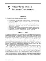
FIVE KEY THEORETICAL RELATIONSHIPS AMONG
SPOT RATE, FORWARD RATES, INFLATION
RATES, AND INTEREST RATES
Expected percentage change
of spot exchange rate of
foreign currency
- 3%

Forward discount or
premium on foreign
currency
- 3%

UFR

IFE

IRP

Interest rate differential
+ 3%

PPP
FE

Expected inflation rate
differential
+ 3%

1


LAW OF ONE PRICE
• If the identical product or service can be:
– Sold in two different markets (perfect substitutability of goods and
services)
– No restrictions exist on the sale (free trade)
– No transportation costs of moving the product between markets
(costless transportation)

※Then the product or service prices should be the same in
both markets
• In a word, perfectly tradable goods or services are subject
to the law of one price
• A primary principle of competitively efficient markets is
that prices of identical products or services will equalize
across them if frictions or transportation costs do not exist

THE LAW OF ONE PRICE

PPP - PURCHASING POWER PARITY
• If the two markets are in two different countries, the
product’s price may be stated in different currency terms
– Price comparison in different markets (countries) would require a
conversion from one currency to the other, e.g.,

P $ × S = P¥
? is P$, the spot exchange rate
where the product price in US dollars
is S (yen per US$), and the price in Japanese yen is P¥

• If these two markets are competitively efficient, i.e., the law
of one price holds, the purchasing power parity (PPP)
exchange rate could be deduced from the relative local
product prices: S = P¥ / P$
– If the price level in the U.S. P$ ↑, then S ↓, which means that the
US$ depreciates

PPP - PURCHASING POWER PARITY
• The absolute version of the PPP theory
– By comparing the prices of identical products denominated in
different competitively efficient currencies, we could
determine the PPP exchange rate

• Example:
Price of wheat in France per bushel (p€) = €3.45
Price of wheat in U.S. per bushel (p$) = $4.15

S€/$ = 0.83215 (s$/€ = 1.2017)

• The hamburger standard or said the Big Mac index is
calculated regularly by The Economist since 1986
Country

Dollar equivalent price of wheat in France = S$/€ x P€
= 1.2017 $/€ x 3.45 € = $4.15

U.S.
Euro area

Big Mac price in US$

Implied PPP
exchange rate

Under (-) / over(+) valuation (FC vs. US$)
relative to the Big Mac index

$3.57

–

–

$5.34
= €3.37×$1.5846/€

$3.57/€3.37=

$1.0593/€

+49.58%
=($1.5846/€ - $1.0593/€) / $1.0593/€

 When law of one price does not hold, supply and demand
forces help restore the equality
※ A Big Mac in the Euro area cost €2.92, and the actual exchange rate is $1.5846/€
※ An alternative to the hamburger standard is the “Starbucks tall-latte index”
introduced by The Economist in 2004

2


/>
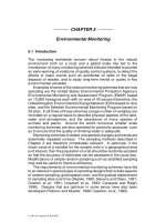
IN-CLASS EXERCISE #1
BIG MAC PRICE
IN LOCAL
CURRENCY

COUNTRY

United State

BIG MAC
PRICE IN $

IMPPLIED PPP
OF $

ACTUAL ER

$2.49

Argentina

Ps2.5

3.13

A$3.00

1.86

Real3.60

2.34

Britain

£1.99

0.69

Canada

C$3.33

1.57

Chile

Ps1,400

655

China

Yuan 10.50

8.28

Australia
Brazil

UNDER/OVER
VALUATION OF
LOCAL CURRENCY

Euro Area

€2.67

0.89

Indonesia

Rupi 16,000

9,430

¥262

130

Japan
Chapter 5

-57% = (3.59 - 8.28):8.28

Local price
$ 2 .9
Food for thought #
May 27th 2004
From The Economist print edition

PPP - PURCHASING POWER PARITY
• Why is the Big Mac a good candidate for the
application of the law of one price?
– The product is nearly identical in each market
– The product is a result of predominantly local materials and
input costs, i.e., its price in each country represents domestic
costs and prices rather than imported ones

• Only a price of single product is not objective enough
to decide the exchange rate
– Replacing the price of a single product with a price index of
a basket of goods, the absolute PPP exchange rate between
two countries can be stated as

S = PI¥ / PI$
7-12

3


PPP - PURCHASING POWER PARITY

EXHIBIT: PPP - PURCHASING POWER PARITY

• Based on the absolute version of the PPP theory, we
can derive relative purchasing power parity (RPPP)
• RPPP is not particularly helpful in determining what
the spot exchange rate today, but that the relative
change in prices between two countries over a period
of time determines the change in the exchange rate
over that period
• More specifically, the spot exchange rate should change
in an equal amount but in the opposite direction to the
difference in inflation rates between two countries
– Thus, the currency with higher (lower) inflation rate will
depreciate (appreciate)

PPP - PURCHASING POWER PARITY
• Given the exchange rate St = Pt¥ / Pt$ (yen per US$) at
time t,
¥
¥
¥
 St+1 

Pt (1   )
(1   )
 St
Pt$ (1   $ )
(1   $ )

• For the indirection quotation of Japanese ¥ for the U.S., the
change of the exchange rate is as follows
¥

St  St+1

St+1


(1   )
(1   $ ) (1   $ )  (1   ¥ )

(1   ¥ )
1  ¥
St
$
(1   )

S t  St

St  St+1
 (1   $ )  (1   ¥ )   $   ¥
St+1

※ For instance, point P represents an equilibrium point where the inflation rate in the
foreign country, Japan, is 4% lower than that in the home country, the U.S.
※ Therefore, RPPP would predict that the Japanese yen would appreciate by 4% per
annum with respect to the U.S. dollars
※ If the domestic country is with a higher inflation rate  prices of domestic products
become relatively expensive  export ↓, import ↑  deficit on current account (and
on BOP)  supply of domestic currency > demand of domestic currency 
domestic currency depreciates

PPP - PURCHASING POWER PARITY
• Empirical testing of PPP and the law of one price has
been done, but has not proved PPP to be accurate in
predicting future exchange rates
• Possible reasons for the poor performance of PPP
– Transportation costs of goods and services are not zero
– Many services are not tradable, e.g., legal services
– Many goods and services are not of the same quality across
countries, reflecting different tastes of consumers in
different countries
– Different tax rules in different countries

+: FC appreciates against DC
–: FC depreciates against DC

※ If π¥ is smaller than π$ (the U.S. is with a higher inflation rate), St+1 is smaller than
St, which indicates the appreciation of Japanese ¥ (depreciation of US$)
※ Furthermore, the percentage change of the PPP exchange rate is proportional to the
difference of the inflation rate (see Exhibit on the next slide)

4


PPP - PURCHASING POWER PARITY

ADJUSTED RER

• Two general conclusions from these studies:
– PPP or RPPP hold well over the very long run but poorly
for shorter time periods
– The theory holds better for countries with relatively high
rates of inflation and underdeveloped capital markets
• A higher inflation rate generates a strong enough pressure to
affect the currency to depreciate
• For countries with underdeveloped capital markets, the
effect of the current account dominates BOP (comparing to
the financial and capital accounts), so there is a closer
relationship between price levels and exchange rates

CPI-VN

CPI-US

NER

1992

100

100.0

10.800

1993

105.2

102.9

1994

114.4

101.8

1995

112.9

102.5

1996

105.5

102.5

1997

103.6

102.7

CPI-VN

CPI-US

RER

1992

100

100.0

10.800

1993

105.2

102.9

1994

114.4

101.8

1995

112.9

102.5

1996

105.5

102.5

1997

103.6

102.7

NOMINAL AND REAL EXCHANGE RATES

ADJUSTED NER

NAÊM

NAÊM

• According to the RPPP, the change of the (nominal)
exchange rate is to offset the change in the differential
growths of price levels between two countries
– For the country with a higher inflation rate, the prices of
products increase inside the country, but due to the

depreciation of the currency of that country, the prices of
products in foreign currency remain the same

• So, the change of the nominal exchange rate will not
affect the relatively competitive power for different
countries
• Only the change of the real exchange rate, which
measures the purchasing power of a currency, will
affect the price competitiveness of a country
18

5


NOMINAL AND REAL EXCHANGE RATES
• The real exchange rate is defined as follows
SR,t = SN,t 

Pf,t
Pd,t

– SR,t: real exchange rate at time t
– SN,t: nominal exchange rate at time t (1 foreign dollar = SN,t
domestic dollars)
– Pf,t: foreign price level at time t relative to the base period at time
0 (Pf,0=100)
– Pd,t: domestic price level at time t relative to the base period at
time 0 (Pd,0=100)
※ If RPPP holds, the magnitude of the increase of the foreign price
level (Pf,t ↑) and the magnitude of the depreciation of the foreign

currency (SN,t ↓) will be the same and offset for each other, so
the real exchange rate will not change

NOMINAL AND REAL EFFECTIVE EXCHANGE RATE
INDICES

• Nominal effective exchange rate index (NEERI) uses
nominal exchange rates to create an index, on a
weighted average basis, of the value of the main
trading currencies over a period of time, which is
defined as follows
n

NEERI t =  Wi  (
i=1

(1/SN,i,t )
(1/SN,i,0 )

 100)

– n: number of major trading currencies for the domestic
country
– Wi: weight of a foreign currency, depending on the trading
volume between the domestic country and that foreign
country
– SN,i,t: nominal exchange rates for the i-th foreign currency at
time t (1/SN,i,t measures the domestic currency value in terms
of foreign currencies)

NOMINAL AND REAL EFFECTIVE EXCHANGE RATE
INDICES

NOMINAL AND REAL EFFECTIVE EXCHANGE
RATE INDICES

• Individual national currencies often need to be
evaluated against all other currency values to
determine relative purchasing power
• The objective is to discover whether a nation’s
exchange rate is “overvalued” or “undervalued” in
terms of PPP
• This problem is often dealt with through the
calculation of exchange rate indices such as the
nominal effective exchange rate index and the real
effective exchange rate index

• Example to calculate NEERI for NT$ against the US$
and Japanese yen (Year 2000 is the base period)
SN,i,2000

SN,i,2008

Trading volume

U.S. (i=1)

1US$=30NT$

1US$=32NT$

NT$ 600 billion

Japan (i=2)

1¥=0.25NT$

1¥=0.2NT$

NT$ 400 billion

NEERI2008 =W1  (

(1/SN,1,2008 )
(1/SN,1,2000 )

 0.6  (

100)  W2  (

(1/SN,2,2008 )
(1/SN,2,2000 )

100)

(1/32)
(1/0.2)
100)  0.4  (
100)  106.25
(1/30)

(1/0.25)

※ From 2000 to 2008, NT$ depreciates against US$ (by 6.25%) and appreciates
against Japanese ¥ (by 25%)
※ From the analysis of NEERI, overall speaking, the nominal exchange rate of NT$
appreciates by 6.25% against the US$ and Japanese ¥

6


NOMINAL AND REAL EFFECTIVE EXCHANGE
RATE INDICES
• Real effective exchange rate index (REERI) indicates
how the weighted average purchasing power of the
domestic currency has changed relative to some
arbitrarily selected base period, which is defined as
follows
n

REERI t =  Wi  (
i=1

(1/SR,i,t )
(1/SR,i,0 )

NOMINAL AND REAL EFFECTIVE EXCHANGE
RATE INDICES

REERI2008 =W1  (

(1/SR,1,2008 )
(1/SR,1,2000 )

 0.6  (

100)  W2  (

(1/SR,2,2008 )
(1/SR,2,2000 )

100)

(1/36.3636)
(1/0.1727)
100)  0.4  (
100)  107.40
(1/30)
(1/0.25)

100)

– SR,i,t: real exchange rates for the i-th foreign currency at time t

※ Overall speaking, the real exchange rate of NT$ appreciates by 7.40% against
the US$ and Japanese ¥
※ In other words, the purchasing power of NT$ increases by 7.40% against the
US$ and Japanese ¥ from 2000 to 2008

NOMINAL AND REAL EFFECTIVE EXCHANGE
RATE INDICES

• Example to calculate REERI for NT$ against the US$
and Japanese yen (Year 2000 is the base period)

U.S. (i=1)

SN,i,2000

SN,i,2008

Price level
in 2000

Price level
in 2008

Trading volume

1US$=30NT$

1US$=32NT$

100

125

NT$ 600 billion

Japan (i=2) 1¥=0.25NT$

1¥=0.2NT$

100

95

NT$ 400 billion

Taiwan

100
110
Pf,1,2000
100
SR,1,2000 = SN,1,2000 
=30 
 30
Pd,2000
100

SR,2,2000 =SN,2,2000 

Pf,2,2000
Pd,2000

SR,1,2008 = SN,1,2008 
SR,2,2008 =SN,2,2008 

Pf,1,2008
Pd,2008

Pf,2,2008
Pd,2008

=0.25 
=32 

100
 0.25
100

NOMINAL AND REAL EFFECTIVE EXCHANGE
RATE INDICES
• The meaning of real effective exchange rate index
(REERI):
– REERIt > REERI0: Real exchange rate of the domestic
currency against foreign currencies appreciates relative to
the base period, so the competitive power of domestic
products decreases relative to the base period
– REERIt < REERI0: Real exchange rate of the domestic
currency against foreign currencies depreciates relative to
the base period, so the competitive power of domestic
products increases relative to the base period

125
 36.3636
110

=0.20 

95

 0.1727
110

7


EXHIBIT 2. REAL EFFECTIVE EXCHANGE RATE INDEXES FOR SOME SELECTED
CURRENCIES (Y2000 = 100)

EXCHANGE RATE PASS-THROUGH

※ From 1981 to 1995, the real exchange rate of Japanese ¥ against foreign currencies appreciates, so the
competitive power of the Japanese products declines
※ From 1995 to 2008, the real exchange rate of Japanese ¥ against foreign currencies depreciates generally,
so the competitive power of the Japanese products increases
※ If the RPPP is true for the long term, i.e., the real exchange rate remains stable due to the offset of the
effects of the changes in nominal exchange rates and inflation rates, the REERI should fluctuate around
100

EXCHANGE RATE PASS-THROUGH
• The degree to which the prices of imported and
exported goods change as a result of exchange rate
changes is termed exchange rate pass-through
• Although PPP implies that all exchange rate changes
are passed through by equivalent changes in prices to
trading partners, empirical researches in the 1980s
questioned this long-held assumption
• For example, a car manufacturer may or may not
adjust pricing of its cars sold in a foreign country if
exchange rates alter the manufacturer’s cost structure

in comparison to the foreign market
• Pass-through can also be partial as there are many
mechanisms by which companies can absorb the
impact of exchange rate changes

※The reason for absorption is trying not to affect the selling volume too much
※The absorption could result from reducing profit margins, cost reductions, or both
※Cost reductions arises from the lower imported price for components and raw
materials to Germany when the euro appreciates

FISHER EFFECT
• The Fisher effect states that nominal interest rates in
each country are equal to the required real rate of
return plus compensation for expected inflation
• Because investors concern about the real returns (i.e.,
the growth of their purchasing power), we would
expect that as inflation increases, investors will
demand higher nominal rates of returns on their
investment
• The nominal interest rate is derived from (1+r) × (1+
π) – 1, and can be reduced to:
i = r + π + rπ  r + π
where i = nominal interest rate, r = real interest rate,
and π = expected inflation

8


FISHER EFFECT
• Because of the arbitrage investment activities among

countries, the real interest rates were to be held
constant among countries, e.g., if the r$ is larger
than the r¥, the capital will flow from Japan to the U.S.
continuously until the r$ equals the r¥
• So, according to the Fisher effect, the nominal interest
rate and the inflation rate have to be adjusted on a
one-for-one basis
• Empirical tests using ex post national inflation rates
and the nominal rates of return of fixed-income
securities have shown the Fisher effect usually exists
for short-maturity government securities (see the next
slide)

FISHER EFFECT

INT’L FISHER EFFECT
• The relationship between the percentage change in
the spot exchange rate over time and the differential
between comparable interest rates in different
national capital markets is known as the
international Fisher effect
• Fisher found that the spot exchange rate should
change in an equal amount but in the opposite
direction to the difference in interest rates
between two countries
– The opposite direction means for a country with lower
(higher) interest rates, its currency will appreciate
(depreciate)

INT’L FISHER EFFECT

• The equation of the international Fisher effect:
i$ – i¥
(1+i$) – (1+i¥)
St  St+1


 i$ – i¥
¥
1+i
1 + i¥
St+1

※ According to the above figure, it is obvious that investors indeed require higher
nominal risk-free rates (T-bill rates) with the increase of higher inflation rates
※However, studies about longer-term government bonds and private sector bonds do
not support the Fisher effect

where i$ and i¥ are the respective nominal interest
rates of the investing period, and St and St+1 are the
spot exchange rates using indirect quotes at the
beginning and the end of that period (¥/$) (if St+1 < St,
it means that the Japanese ¥ appreciates)
• According to the above equation, the currency with
lower interest rate will appreciate
– If i$ =6% and i¥ =4%, St+1 is expected to be smaller than St
by 2%, which means that the Japanese ¥ should appreciate
about 2% per year

9

CURRENCY FORECATING

INT’L FISHER EFFECT
• The unrestricted capital flows will see the
opportunity around the world and make the
international Fisher effect to be true
• For example, if i$ =6% and i¥ =5%, and the
Japanese ¥ is expected to appreciate 2%, the
unrestricted capital will flow from the U.S. to Japan
to earn 7% (=5% + 2%) return. This activity will
increase the money supply in the Japanese
economy and thus reduce the i¥ until it becomes 4%
(thus the international Fisher effect holds again)

•

Currency forecasting can lead to consistent profits only if the forecaster meets at
least one of the following four criteria.
– Has exclusive use of a superior forecasting model
– Has consistent access to information before other investors
– Exploits small, temporary deviations from equilibrium
– can predict the nature of government intervention in the foreign exchange

•

As a general rule, in a fixed rate system, the forecaster must focus on the
governmental decision-making structure because the decision to devalue or revalue
at a given time is clearly political.

•

In case of floating system, currency forecasting have the choice of using either
market or model-based forecasts, neither of which guarantees success.

INT’L FISHER EFFECT #
• The international Fisher effect vs. the Relative
Purchase Power Parity (RPPP)
St  St+1 $ ¥
¥
 i  i  (r $   $ )  (r ¥   )
St+1
  $  ¥

By force of the international
arbitrage, real rates of return
between markets should be
equal, i.e., r$=r¥

※ The international Fisher effect and the RPPP is consistent if the Fisher effect
is valid
※ The only difference is that in the international Fisher effect, the interest rate,
i, is applied to a future time period and thus the inflation rate, π, is the
expected inflation rate

FORECASTING EXCHANGE RATES: EFFICIENT
MARKETS APPROACH
• Financial markets are efficient if prices reflect all available and
relevant information.
• The efficient market hypothesis (Prof. Eugene Fama)

• If this is true, exchange rates will only change when new
information arrives, thus:
St = E[St+1]
The random walk hypothesis suggest that today’s ER is the
best predictor of tomorrow’s ER
Ft = E[St+1| It]
• Predicting exchange rates using the efficient markets approach
is affordable and is hard to beat.

※ In the RPPP, however, the inflation rate, π, is ex post, i.e., only at the end of
the period, the inflation rate for that period is known, and thus the exchange
rate should
7-38 change in response to the realized inflation rate

10


FORECASTING EXCHANGE RATES:
FUNDAMENTAL APPROACH
• Involves econometrics to develop models that use a
variety of explanatory variables. This involves three
steps:
– Step 1: Estimate the structural model.
– Step 2: Estimate future parameter values.
– Step 3: Use the model to develop forecasts.

FORECASTING EXCHANGE RATES: TECHNICAL
APPROACH
• Technical analysis looks for patterns in the past
behavior of exchange rates.

• Clearly it is based upon the premise that history
repeats itself.

• The downside is that fundamental models do not work
any better than the forward rate model or the random
walk model.

FORECASTING EXCHANGE RATES:
FUNDAMENTAL APPROACH #

MOVING AVERAGE CROSSOVER RULE: GOLDEN
CROSS vs DEATH CROSS

s    1 (m  m* )   2 (  * )   3 ( y *  y )  
•
•
•
•
•
•

S: natural logarithm of spot ER
m-m*: natural logarithm of domestic/foreign money supply
 - *: natural logarithm of domestic/foreign velocity of money
y-y*: natural logarithm of domestic/foreign output
: random error term, with zero mean
, : model parameter

LMA: Long-term Moving Average

SMA: Short-term Moving Average

11


HEAD AND SHOULDERS PATTERN: A REVERSAL SIGNAL

R

MAE ( S )
MAE ( F )

1
MAE   i Pi  Ai
N

MAE(S): mean absolute forecast error of a forecasting service
MAE(F): mean absolute forecast error of the forward exchange rate as a predictor

PERFORMANCE OF THE FORECASTERS
• Forecasting is difficult, especially with regard to the
future.
• As a whole, forecasters cannot do a better job of
forecasting future exchange rates than the forecast
implied by the forward rate.
• The founder of Forbes Magazine once said, “You can
make more money selling financial advice than
following it.”

R

MSE ( B )
MSE ( S )

MSE(B)
MSE(B): mean squared forecast error of a bank
MSE(S): mean squared forecast error of the spot exchange rate

12


INVESTOR PSYCHOLOGY AND BANDWAGON EFFECTS

How are exchange rates influenced by investor
psychology?
The bandwagon effect occurs when expectations on the
part of traders turn into self-fulfilling prophecies, and
traders join the bandwagon and move exchange rates
based on group expectations
• Governmental intervention can prevent the bandwagon from
starting, but is not always effective

Impact of Inflation on an MNC’s Value
Effect of Inflation

m
E CFj , t  E ER j , t 
n 



Value =   j 1

t
1  k 
t =1 



E (CFj,t ) = expected cash flows in currency j to be received
by the U.S. parent at the end of period t
E (ERj,t ) = expected exchange rate at which currency j can
be converted to dollars at the end of period t
k
= weighted average cost of capital of the parent

SUMMARY
 Relative monetary growth, relative inflation rates, and nominal
interest rate differentials are all moderately good predictors of
long-run changes in exchange rates, but poor predictors of
short term changes
 So, international businesses should pay attention to countries’
differing monetary growth, inflation, and interest rates

13