Handbook of food engineering 2nd ed d heldman 2007
Bạn đang xem bản rút gọn của tài liệu. Xem và tải ngay bản đầy đủ của tài liệu tại đây (14.12 MB, 1,038 trang )
Heldman: “dk2202_c000” — 2006/10/9 — 20:06 — page i — #1
Heldman: “dk2202_c000” — 2006/10/9 — 20:06 — page ii — #2
Heldman: “dk2202_c000” — 2006/10/9 — 20:06 — page iii — #3
Heldman: “dk2202_c000” — 2006/10/9 — 20:06 — page iv — #4
Preface
The primary mission of the second edition of the Handbook of Food Engineering is the same as the
first. The most recent information needed for efficient design and development of processes used
in the manufacturing of food products has been assembled, along with the traditional background on
these processes. The audience for this handbook includes three groups: (1) practicing engineers in
the food and related industries, (2) the student preparing for a career as a food engineer, and (3) other
scientists and technologists seeking information about processes and the information needed in design
and development of these processes. For the practicing engineer, the handbook assembles information
needed for the design and development of a given process. For the student, the handbook becomes
the primary reference needed to supplement textbooks used in the teaching of process design and
development concepts. Other scientists and technologists should use the handbook to locate important
information and physical data related to foods and food ingredients.
As in the first edition, the handbook assembles the most recent information on thermophysical
properties of foods, rate constants about changes in food components during a process, and illustrations of the use of these properties and constants in process design. Researchers will be able to
use the information as a guide in establishing the direction of future research on thermophysical
properties and rate constants. In this edition, an appendix has been created to assemble tables and
figures containing property data needed for the design of processes described in various chapters of
the handbook.
Although the first three chapters focus primarily on properties of food and food ingredients,
the chapters that follow are organized according to traditional unit operations associated with the
manufacturing of foods. Two key chapters cover the basic concepts of transport and storage of liquids
and solids, and the heating and cooling of foods and food ingredients. An additional background
chapter focuses on basic concepts of mass transfer in foods. More specific unit operations on freezing,
concentration, dehydration, thermal processing, and extrusion are discussed and analyzed in separate
chapters. The chapter on membrane processes deals with liquid food concentration but provides the
basis for other applications of membranes in food processing. The final chapters of the handbook
cover the important topics of packaging and cleaning and sanitation.
The editors of this handbook hope that the information presented will continue to contribute to
the evolution of food engineering as an interface between engineering and other food sciences. As
demands for safe, high quality, nutritious and convenient foods continue to increase, the needs for
the concepts presented will become more critical. In the near future, the applications of new science
from molecular biology, nanotechnology, and nutritional biochemistry in food manufacturing will
increase, and the role of engineering in process design and scale-up will be even more visible. At
the same time, new process technologies will continue to emerge and require input from engineers
for application, design, and development in food manufacturing. Ultimately, the use of engineering
concepts should lead to the highest quality food products at the lowest possible cost.
The editors wish to acknowledge the authors and their significant contributions to the second
edition of this handbook. These authors are among the leading scientists and engineers in the field
Heldman: “dk2202_c000” — 2006/10/9 — 20:06 — page v — #5
of food engineering. We are pleased to be associated with their contributions to this field and to the
handbook.
Dennis R. Heldman
Daryl B. Lund
Heldman: “dk2202_c000” — 2006/10/9 — 20:06 — page vi — #6
Editors
Dennis R. Heldman is a principal of Heldman Associates in Weston, Florida. He has been professor
of food process engineering at Rutgers, The State University of New Jersey, the University of
Missouri and Michigan State University. In addition, he has industry experience at the Campbell
Soup Company, the National Food Processors Association and the Weinberg Consulting Group.
Dr. Heldman is the author or co-author of over 140 journal articles, and the author, co-author or
editor of over 10 textbooks, handbooks and encyclopedias. He is a fellow of the Institute of Food
Technologists and the American Society of Agricultural Engineers. He served as president of the
IFT, the Society for Food Science and Technology, an organization with over 20,000 members, from
2006–2007, and was elected fellow in the International Academy of Food Science & Technology in
2006. Dr. Heldman was awarded a BS (1960) and an MS (1962) from The Ohio State University,
and a PhD (1965) from Michigan State University.
Darryl B. Lund earned a BS (1963) in mathematics and a PhD (1968) in food science with a minor
in chemical engineering at the University of Wisconsin-Madison. During 21 years at the University
of Wisconsin, he was a professor of food engineering in the food science department serving as chair
of the department from 1984–1987. He has contributed over 150 scientific papers, edited 5 books,
and co-authored one major textbook in the area of simultaneous heat and mass transfer in foods,
kinetics of reactions in foods, and food processing.
In 1988 he continued his administrative responsibilities by chairing the Department of Food
Science at Rutgers University, and from December 1989 through July 1995 served as the executive
dean of Agriculture and Natural Resources with responsibilities for teaching, research and extension
at Rutgers University. In that position, among other achievements, he initiated a rigorous strategic
planning process for Cook College and the New Jersey Agricultural Experiment Station, streamlined
administrative services, fostered a review of the undergraduate curriculum and encouraged the faculty
to develop a social contact for undergraduate instruction.
In August 1995, he joined the Cornell University faculty as the Ronald P. Lynch Dean of Agriculture and Life Sciences. During his tenure as dean of CALS, he initiated a strategic positioning
process for the college that guided the college through 20% downsizing, promoted the Agriculture
Initiative to gain increased state support for the Agricultural Experiment Station and Cooperative
Extension, supported an initiative in genomics and overhaul of the biological sciences, fostered a
review of undergraduate programs that led to major changes, and supported the adoption of electronic
technologies for undergraduate teaching and distance education. In July 2000, Dr. Lund returned to
the Department of Food Science as professor of food engineering.
In January 2001, Dr. Lund became the executive director of the North Central Regional Association of State Agricultural Experiment Station Directors. In this position he facilitates interstate
collaboration on research and a greater integration between research and extension in the twelve-state
region.
Among many awards in recognition of personal achievement, he is a recipient of the
ASAE/DFISA Food Engineering Award, the IFT International Award and Carl R. Fellers Award,
and the Irving Award from the American Distance Education Consortium. He is an elected fellow of
the Institute of Food Technologists, elected fellow of the Institute of Food Science and Technology
(UK), and charter inductee in the International Academy of Food Science and Technology.
Heldman: “dk2202_c000” — 2006/10/9 — 20:06 — page vii — #7
Heldman: “dk2202_c000” — 2006/10/9 — 20:06 — page viii — #8
Contributors
Osvaldo Campanella
Purdue University
West Lafayette, Indiana
Leon Levine
Leon Levine and Associates, Inc.
Albuquerque, New Mexico
Munir Cheryan
University of Illinois at Urbana-Champaign
Urbana, Illinois
Robert C. Miller
Consulting Engineer
Auburn, New York
Hulya Dogan
The State University of New Jersey, Rutgers
New Brunswick, New Jersey
Ken R. Morison
University of Canterbury
Christchurch, New Zealand
Vassilis Gekas
Technical University of Crete
Chania, Greece
Ganesan Narsimhan
Purdue University
West Lafayette, Indiana
Albrecht Graßhoff
Bundesanstalt für Milchforschung
Kiel, Germany
Martin R. Okos
Purdue University
West Lafayette, Indiana
Bengt Hallström
University of Lund
Lund, Sweden
Erwin A. Plett
Sello Verde Ingenieria Ambiental S.A.
Santiago, Chile
Richard W. Hartel
University of Wisconsin
Madison, Wisconsin
M.A. Rao
Cornell University
Ithaca, New York
James G. Hawkes
Nutriscience Technologies, Inc.
Naperville, Illinois
Anne Marie Romulus
Université Paul Sabatier
Toulouse, France
Dennis R. Heldman
Heldman Associates
Weston, Florida
Yrjö H. Roos
University College
Cork, Ireland
Jozef L. Kokini
The State University of New Jersey, Rutgers
New Brunswick, New Jersey
R. Paul Singh
University of California
Davis, California
John M. Krochta
University of California
Davis, California
Rakesh K. Singh
Purdue University
West Lafayette, Indiana
Heldman: “dk2202_c000” — 2006/10/9 — 20:06 — page ix — #9
Ingegerd Sjöholm
University of Lund
Lund, Sweden
Ricardo Villota
Kraft Foods
Glenview, Illinois
Arthur Teixeira
University of Florida
Gainesville, Florida
A.C. Weitnauer
Purdue University
West Lafayette, Indiana
Heldman: “dk2202_c000” — 2006/10/9 — 20:06 — page x — #10
Table of Contents
Chapter 1 Rheological Properties of Foods . . . . . . . . . . . . . . . . . . . . . . . . . . . . . . . . . . . . . . . . . . . . . . . . . . . . .
Hulya Dogan and Jozef L. Kokini
1
Chapter 2 Reaction Kinetics in Food Systems . . . . . . . . . . . . . . . . . . . . . . . . . . . . . . . . . . . . . . . . . . . . . . . . . . 125
Ricardo Villota and James G. Hawkes
Chapter 3 Phase Transitions and Transformations in Food Systems . . . . . . . . . . . . . . . . . . . . . . . . . . . 287
Yrjö H. Roos
Chapter 4 Transport and Storage of Food Products . . . . . . . . . . . . . . . . . . . . . . . . . . . . . . . . . . . . . . . . . . . . . 353
M.A. Rao
Chapter 5 Heating and Cooling Processes for Foods . . . . . . . . . . . . . . . . . . . . . . . . . . . . . . . . . . . . . . . . . . . 397
R. Paul Singh
Chapter 6 Food Freezing . . . . . . . . . . . . . . . . . . . . . . . . . . . . . . . . . . . . . . . . . . . . . . . . . . . . . . . . . . . . . . . . . . . . . . . . . 427
Dennis R. Heldman
Chapter 7 Mass Transfer in Foods . . . . . . . . . . . . . . . . . . . . . . . . . . . . . . . . . . . . . . . . . . . . . . . . . . . . . . . . . . . . . . . 471
Bengt Hallström, Vassilis Gekas, Ingegerd Sjöholm, and Anne Marie Romulus
Chapter 8 Evaporation and Freeze Concentration . . . . . . . . . . . . . . . . . . . . . . . . . . . . . . . . . . . . . . . . . . . . . . 495
Ken R. Morison and Richard W. Hartel
Chapter 9 Membrane Concentration of Liquid Foods . . . . . . . . . . . . . . . . . . . . . . . . . . . . . . . . . . . . . . . . . . 553
Munir Cheryan
Chapter 10 Food Dehydration . . . . . . . . . . . . . . . . . . . . . . . . . . . . . . . . . . . . . . . . . . . . . . . . . . . . . . . . . . . . . . . . . . . 601
Martin R. Okos, Osvaldo Campanella, Ganesan Narsimhan, Rakesh K. Singh,
and A.C. Weitnauer
Chapter 11 Thermal Processing of Canned Foods . . . . . . . . . . . . . . . . . . . . . . . . . . . . . . . . . . . . . . . . . . . . . . 745
Arthur Teixeira
Chapter 12 Extrusion Processes . . . . . . . . . . . . . . . . . . . . . . . . . . . . . . . . . . . . . . . . . . . . . . . . . . . . . . . . . . . . . . . . . 799
Leon Levine and Robert C. Miller
Chapter 13 Food Packaging . . . . . . . . . . . . . . . . . . . . . . . . . . . . . . . . . . . . . . . . . . . . . . . . . . . . . . . . . . . . . . . . . . . . . . 847
John M. Krochta
Heldman: “dk2202_c000” — 2006/10/9 — 20:06 — page xi — #11
Chapter 14 Cleaning and Sanitation . . . . . . . . . . . . . . . . . . . . . . . . . . . . . . . . . . . . . . . . . . . . . . . . . . . . . . . . . . . . . 929
Erwin A. Plett and Albrecht Graßhoff
Appendix . . . . . . . . . . . . . . . . . . . . . . . . . . . . . . . . . . . . . . . . . . . . . . . . . . . . . . . . . . . . . . . . . . . . . . . . . . . . . . . . . . . . . . . . . . . 977
Index . . . . . . . . . . . . . . . . . . . . . . . . . . . . . . . . . . . . . . . . . . . . . . . . . . . . . . . . . . . . . . . . . . . . . . . . . . . . . . . . . . . . . . . . . . . . . . . . 1009
Heldman: “dk2202_c000” — 2006/10/9 — 20:06 — page xii — #12
1
Rheological Properties
of Foods
Hulya Dogan and Jozef L. Kokini
CONTENTS
1.1
1.2
1.3
1.4
1.5
Introduction . . . . . . . . . . . . . . . . . . . . . . . . . . . . . . . . . . . . . . . . . . . . . . . . . . . . . . . . . . . . . . . . . . . . . . . . . . . . . . . . . .
Basic Concepts . . . . . . . . . . . . . . . . . . . . . . . . . . . . . . . . . . . . . . . . . . . . . . . . . . . . . . . . . . . . . . . . . . . . . . . . . . . . . . .
1.2.1 Stress and Strain . . . . . . . . . . . . . . . . . . . . . . . . . . . . . . . . . . . . . . . . . . . . . . . . . . . . . . . . . . . . . . . . . . . . .
1.2.2 Classification of Materials . . . . . . . . . . . . . . . . . . . . . . . . . . . . . . . . . . . . . . . . . . . . . . . . . . . . . . . . . .
1.2.3 Types of Deformation . . . . . . . . . . . . . . . . . . . . . . . . . . . . . . . . . . . . . . . . . . . . . . . . . . . . . . . . . . . . . . .
1.2.3.1 Shear Flow . . . . . . . . . . . . . . . . . . . . . . . . . . . . . . . . . . . . . . . . . . . . . . . . . . . . . . . . . . . . . . . .
1.2.3.2 Extensional (Elongational) Flow . . . . . . . . . . . . . . . . . . . . . . . . . . . . . . . . . . . . . . . . .
1.2.3.3 Volumetric Flows . . . . . . . . . . . . . . . . . . . . . . . . . . . . . . . . . . . . . . . . . . . . . . . . . . . . . . . . .
1.2.4 Response of Viscous and Viscoelastic Materials in Shear and Extension . . . . . . . .
1.2.4.1 Stress Relaxation . . . . . . . . . . . . . . . . . . . . . . . . . . . . . . . . . . . . . . . . . . . . . . . . . . . . . . . . . .
1.2.4.2 Creep . . . . . . . . . . . . . . . . . . . . . . . . . . . . . . . . . . . . . . . . . . . . . . . . . . . . . . . . . . . . . . . . . . . . . .
1.2.4.3 Small Amplitude Oscillatory Measurements . . . . . . . . . . . . . . . . . . . . . . . . . . . .
1.2.4.4 Interrelations between Steady Shear and Dynamic Properties . . . . . . . . . .
Methods of Measurement . . . . . . . . . . . . . . . . . . . . . . . . . . . . . . . . . . . . . . . . . . . . . . . . . . . . . . . . . . . . . . . . . . .
1.3.1 Shear Measurements . . . . . . . . . . . . . . . . . . . . . . . . . . . . . . . . . . . . . . . . . . . . . . . . . . . . . . . . . . . . . . . .
1.3.2 Small Amplitude Oscillatory Measurements . . . . . . . . . . . . . . . . . . . . . . . . . . . . . . . . . . . . . . .
1.3.3 Extensional Measurements . . . . . . . . . . . . . . . . . . . . . . . . . . . . . . . . . . . . . . . . . . . . . . . . . . . . . . . . . .
1.3.4 Stress Relaxation . . . . . . . . . . . . . . . . . . . . . . . . . . . . . . . . . . . . . . . . . . . . . . . . . . . . . . . . . . . . . . . . . . . .
1.3.5 Creep Recovery . . . . . . . . . . . . . . . . . . . . . . . . . . . . . . . . . . . . . . . . . . . . . . . . . . . . . . . . . . . . . . . . . . . . . .
1.3.6 Transient Shear Stress Development . . . . . . . . . . . . . . . . . . . . . . . . . . . . . . . . . . . . . . . . . . . . . . .
1.3.7 Yield Stresses . . . . . . . . . . . . . . . . . . . . . . . . . . . . . . . . . . . . . . . . . . . . . . . . . . . . . . . . . . . . . . . . . . . . . . . .
Constitutive Models . . . . . . . . . . . . . . . . . . . . . . . . . . . . . . . . . . . . . . . . . . . . . . . . . . . . . . . . . . . . . . . . . . . . . . . . .
1.4.1 Simulation of Steady Rheological Data . . . . . . . . . . . . . . . . . . . . . . . . . . . . . . . . . . . . . . . . . . . .
1.4.2 Linear Viscoelastic Models . . . . . . . . . . . . . . . . . . . . . . . . . . . . . . . . . . . . . . . . . . . . . . . . . . . . . . . . .
1.4.2.1 Maxwell Model . . . . . . . . . . . . . . . . . . . . . . . . . . . . . . . . . . . . . . . . . . . . . . . . . . . . . . . . . . .
1.4.2.2 Voigt Model . . . . . . . . . . . . . . . . . . . . . . . . . . . . . . . . . . . . . . . . . . . . . . . . . . . . . . . . . . . . . . .
1.4.2.3 Multiple Element Models. . . . . . . . . . . . . . . . . . . . . . . . . . . . . . . . . . . . . . . . . . . . . . . . .
1.4.2.4 Mathematical Evolution of Nonlinear Constitutive Models . . . . . . . . . . . .
1.4.3 Nonlinear Constitutive Models . . . . . . . . . . . . . . . . . . . . . . . . . . . . . . . . . . . . . . . . . . . . . . . . . . . . .
1.4.3.1 Differential Constitutive Models . . . . . . . . . . . . . . . . . . . . . . . . . . . . . . . . . . . . . . . . .
1.4.3.2 Integral Constitutive Models . . . . . . . . . . . . . . . . . . . . . . . . . . . . . . . . . . . . . . . . . . . . .
Molecular Information from Rheological Measurements. . . . . . . . . . . . . . . . . . . . . . . . . . . . . . . . . .
1.5.1 Dilute Solution Molecular Theories . . . . . . . . . . . . . . . . . . . . . . . . . . . . . . . . . . . . . . . . . . . . . . . .
1.5.2 Concentrated Solution Theories . . . . . . . . . . . . . . . . . . . . . . . . . . . . . . . . . . . . . . . . . . . . . . . . . . . .
1.5.2.1 The Bird–Carreau Model . . . . . . . . . . . . . . . . . . . . . . . . . . . . . . . . . . . . . . . . . . . . . . . . .
1.5.2.2 The Doi–Edwards Model . . . . . . . . . . . . . . . . . . . . . . . . . . . . . . . . . . . . . . . . . . . . . . . . .
2
3
3
4
4
4
6
9
10
10
11
12
15
18
19
25
27
30
34
36
40
41
42
47
49
52
53
57
58
58
63
67
67
71
71
75
1
Heldman: “dk2202_c001” — 2006/9/21 — 15:44 — page 1 — #1
2
Handbook of Food Engineering
1.5.3
Understanding Polymeric Properties from Rheological Properties . . . . . . . . . . . . . . .
1.5.3.1 Gel Point Determination . . . . . . . . . . . . . . . . . . . . . . . . . . . . . . . . . . . . . . . . . . . . . . . . . .
1.5.3.2 Glass Transition Temperature and the Phase Behavior. . . . . . . . . . . . . . . . . .
1.5.3.3 Networking Properties . . . . . . . . . . . . . . . . . . . . . . . . . . . . . . . . . . . . . . . . . . . . . . . . . . . .
1.6 Use of Rheological Properties in Practical Applications . . . . . . . . . . . . . . . . . . . . . . . . . . . . . . . . . .
1.6.1 Sensory Evaluations . . . . . . . . . . . . . . . . . . . . . . . . . . . . . . . . . . . . . . . . . . . . . . . . . . . . . . . . . . . . . . . . .
1.6.2 Molecular Conformations . . . . . . . . . . . . . . . . . . . . . . . . . . . . . . . . . . . . . . . . . . . . . . . . . . . . . . . . . . .
1.6.3 Product and Process Characterization . . . . . . . . . . . . . . . . . . . . . . . . . . . . . . . . . . . . . . . . . . . . . .
1.7 Numerical Simulation of Flows . . . . . . . . . . . . . . . . . . . . . . . . . . . . . . . . . . . . . . . . . . . . . . . . . . . . . . . . . . . . .
1.7.1 Numerical Simulation Techniques. . . . . . . . . . . . . . . . . . . . . . . . . . . . . . . . . . . . . . . . . . . . . . . . . .
1.7.2 Selection of Constitutive Models . . . . . . . . . . . . . . . . . . . . . . . . . . . . . . . . . . . . . . . . . . . . . . . . . . .
1.7.3 Finite Element Simulations . . . . . . . . . . . . . . . . . . . . . . . . . . . . . . . . . . . . . . . . . . . . . . . . . . . . . . . . .
1.7.3.1 FEM Techniques for Viscoelastic Fluid Flows . . . . . . . . . . . . . . . . . . . . . . . . . .
1.7.3.2 FEM Simulations of Flow in an Extruder. . . . . . . . . . . . . . . . . . . . . . . . . . . . . . . .
1.7.3.3 FEM Simulations of Flow in Model Mixers . . . . . . . . . . . . . . . . . . . . . . . . . . . . .
1.7.3.4 FEM Simulations of Mixing Efficiency. . . . . . . . . . . . . . . . . . . . . . . . . . . . . . . . . .
1.7.4 Verification and Validation of Mathematical Simulations . . . . . . . . . . . . . . . . . . . . . . . .
1.8 Concluding Remarks . . . . . . . . . . . . . . . . . . . . . . . . . . . . . . . . . . . . . . . . . . . . . . . . . . . . . . . . . . . . . . . . . . . . . . . .
References . . . . . . . . . . . . . . . . . . . . . . . . . . . . . . . . . . . . . . . . . . . . . . . . . . . . . . . . . . . . . . . . . . . . . . . . . . . . . . . . . . . . . . . . . .
77
77
81
85
88
88
91
95
96
96
98
98
99
100
101
105
111
114
115
1.1 INTRODUCTION
Rheological properties are important to the design of flow processes, quality control, storage and
processing stability measurements, predicting texture, and learning about molecular and conformational changes in food materials (Davis, 1973). The rheological characterization of foods provides
important information for food scientists, ingredient selection strategies to design, improve, and
optimize their products, to select and optimize their manufacturing processes, and design packaging
and storage strategies. Rheological studies become particularly useful when predictive relationships
for rheological properties of foods can be developed which start from the molecular architecture of
the constituent species.
Reliable and accurate steady rheological data are necessary to design continuous-flow processes, select and size pumps and other fluid-moving machinery and to evaluate heating rates during
engineering operations which include flow processes such as aseptic processing and concentration
(Holdsworth, 1971; Sheath, 1976), and to estimate velocity, shear, and residence-time distribution
in food processing operations including extrusion and continuous mixing.
Viscoelastic properties are also useful in processing and storage stability predictions. For
example, during extrusion, viscoelastic properties of cereal flour doughs affect die swell and extrudate expansion. In batch mixing, elasticity is responsible for the rod climbing phenomenon, also
known as the Weissenberg effect (Bird et al., 1987). To allow for elastic recovery of dough during
cookie making, the dough is cut in the form of an ellipse which relaxes into a perfect circle.
Creep and small-amplitude oscillatory measurements are useful in understanding the role of constituent ingredients on the stability of oil-in-water emulsions. Steady shear and creep measurements
help identify the effect of ingredients that have stabilizing ability, such as gums, proteins, or other
surface-active agents (Fischbach and Kokini, 1984).
Dilute solution viscoelastic properties of biopolymeric materials such as carbohydrates and protein can be used to characterize their three-dimensional configuration in solution. Their configuration
affects their functionality in many food products. It is possible to predict better and improve the flow
behavior of food polymers through an understanding of how the molecular structure of polymers
affects their rheological properties (Liguori, 1985). Examples can be found in the improvement of
Heldman: “dk2202_c001” — 2006/9/21 — 15:44 — page 2 — #2
Rheological Properties of Foods
3
2
22
12
21
23
11
1
13
1-plane
3
FIGURE 1.1 Stress components on a cubical material element.
the consistency and stability of emulsions by using polymers with enhanced surface activity and
greater viscosity and elasticity.
This chapter will review recent advances in basic rheological concepts, methods of measurement,
molecular theories, linear and nonlinear constitutive models, and numerical simulation of viscoelastic
flows.
1.2 BASIC CONCEPTS
1.2.1 STRESS AND STRAIN
Rheology is the science of the deformation and flow of matter. Rheological properties define the
relationship between stress and strain/strain rate in different types of shear and extensional flows. The
stress is defined as the force F acting on a unit area A. Since both force and area have directional as
well as magnitude characteristics, stress is a second order tensor and typically has nine components.
Strain is a measure of deformation or relative displacement and is determined by the displacement
gradient. Since displacement and its relative change both have directional properties, strain is also a
second order tensor with nine components.
A rheological measurement is conducted on a given material by imposing a well-defined stress
and measuring the resulting strain or strain rate or by imposing a well-defined strain or strain rate and
by measuring the stress developed. The relationship between these physical events leads to different
kinds of rheological properties.
When a force F is applied to a piece of material (Figure 1.1), the total stress acting on any
infinitesimal element is composed of two fundamental classes of stress components (Darby, 1976):
Normal stress components, applied perpendicularly to the plane (τ11 , τ22 , τ33 )
Shear stress components, applied tangentially to the plane (τ12 , τ13 , τ21 , τ23 , τ31 , τ32 )
There are a total of nine stress components acting on an infinitesimal element (i.e., two shear
components and one normal stress component acting on each of the three planes). Individual stress
components are referred to as τij , where i refers to the plane the stress acts on, and j indicates the
direction of stress component (Bird et al., 1987). The stress tensor can be written as a matrix of nine
components as follows:
τ11
τ = τ21
τ31
τ12
τ22
τ32
τ13
τ23
τ33
Heldman: “dk2202_c001” — 2006/9/21 — 15:44 — page 3 — #3
4
Handbook of Food Engineering
In general, the stress tensor in the deformation of an incompressible material is described by three
shear stresses and two normal stress differences:
Shear stresses:
τ12 (=τ21 )
τ13 (=τ31 )
Normal stress differences: N1 = τ11 − τ22
τ23 (=τ32 )
N2 = τ22 − τ33
1.2.2 CLASSIFICATION OF MATERIALS
Rheological properties of materials are the result of their stress-strain behavior. Ideal solid (elastic)
and ideal fluid (viscous) behaviors represent two extreme responses of a material (Darby, 1976).
An ideal solid material deforms instantaneously when a load is applied. It returns to its original
configuration instantaneously (complete recovery) upon removal of the load. Ideal elastic materials
obey Hooke’s law, where the stress (τ ) is directly proportional to the strain (γ ). The proportionality
constant (G) is called the modulus.
τ = Gγ
An ideal fluid deforms at a constant rate under an applied stress, and the material does not
regain its original configuration when the load is removed. The flow of a simple viscous material is
described by Newton’s law, where the shear stress (τ ) is directly proportional the shear rate (γ˙ ). The
proportionality constant (η) is called the Newtonian viscosity.
τ = ηγ˙
Most food materials exhibit characteristics of both elastic and viscous behavior and are called
viscoelastic. If viscoelastic properties are strain and strain rate independent, then these materials
are referred to as linear viscoelastic materials. On the other hand if they are strain and strain rate
dependent, than they are referred to as nonlinear viscoelastic materials (Ferry, 1980; Bird et al.,
1987; Macosko, 1994).
A simple and classical approach to describe the response of a viscoelastic material is using
mechanical analogs. Purely elastic behavior is simulated by springs and purely viscous behavior is
simulated using dashpots. The Maxwell and Voigt models are the two simplest mechanical analogs
of viscoelastic materials. They simulate a liquid (Maxwell) and a solid (Voigt) by combining a
spring and a dashpot in series or in parallel, respectively. These mechanical analogs are the building
blocks of constitutive models as discussed in Section 1.4 in detail.
1.2.3 TYPES OF DEFORMATION
1.2.3.1 Shear Flow
One of the most useful types of deformation for rheological measurements is simple shear. In simple
shear, a material element is placed between two parallel plates (Figure 1.2) where the bottom plate is
stationary and the upper plate is displaced in x-direction by x by applying a force F tangentionally
to the surface A. The velocity profile in simple shear is given by the following velocity components:
vx = γ˙ y,
vy = 0,
and
vz = 0
The corresponding shear stress is given as:
τ=
F
A
Heldman: “dk2202_c001” — 2006/9/21 — 15:44 — page 4 — #4
Rheological Properties of Foods
5
A
F
∆y
vx
y
x
FIGURE 1.2 Shear flow.
If the relative displacement at any given point
γ =
y is
x, then the shear strain is given by
x
y
If the material is a fluid, force applied tangentially to the surface will result in a constant velocity vx
in x-direction. The deformation is described by the strain rate (γ˙ ), which is the time rate of change
of the shear strain:
γ˙ =
dγ
d
=
dt
dt
x
y
=
dvx
dy
Shear strain defines the displacement gradient in simple shear. The displacement gradient is the
relative displacement of two points divided by the initial distance between them. For any continuous
medium the displacement gradient tensor is given as:
∂u1
∂x1
∂u
∂ui
2
=
∂x1
∂xj
∂u3
∂x1
∂u1
∂x2
∂u2
∂x2
∂u3
∂x2
∂u1
∂x3
∂u2
∂x3
∂u3
∂x3
A nonzero displacement gradient may represent pure rotation, pure deformation, or both (Darby,
1976). Thus, each displacement component has two parts:
∂ui
1
=
∂xj
2
∂uj
∂ui
+
∂xj
∂xi
+
1
2
Pure deformation
∂uj
∂ui
−
∂xj
∂xi
Pure rotation
Then the strain tensor (eij ) can be defined as:
eij =
∂uj
∂ui
+
∂xj
∂xi
Similarly, the rotation tensor (rij ) can be defined as:
rij =
∂uj
∂ui
−
∂xi
∂xj
Heldman: “dk2202_c001” — 2006/9/21 — 15:44 — page 5 — #5
6
Handbook of Food Engineering
In simple shear, there is only one nonzero displacement gradient component that contributes to
both strain and rotation tensors.
∂ux
0
0
0 1 0
∂ui
∂y
= dux 0 0 0
=
0
0
0
∂xj
dy 0 0 0
0
0
0
The time derivative of the strain tensor gives the rate of strain tensor (
ij
=
∂
∂
(eij ) =
∂t
∂t
∂uj
∂ui
+
∂xj
∂xi
=
ij ):
∂vj
∂vi
+
∂xj
∂xi
Similarly, time derivative of the rotation tensor gives the vorticity tensor (
ij
=
ij ):
∂νj
∂
∂νi
(rij ) =
−
∂t
∂xi
∂xj
Simple shear flow, or viscometric flow, serves as the basis for many rheological measurement
techniques (Bird et al., 1987). The stress tensor in simple shear flow is given as:
0
τ = τ21
0
τ12
0
0
0
0
0
There are three shear rate dependent material functions used to describe material properties in
simple shear flow:
τ12
γ˙
τ11 − τ22
N1
First normal stress coefficient:
ψ1 (γ˙ ) =
= 2
2
γ˙
γ˙
τ22 − τ33
N2
Second normal stress coefficient: ψ2 (γ˙ ) =
= 2
2
γ˙
γ˙
Viscosity:
µ(γ˙ ) =
Among the viscometric functions, viscosity is the most important parameter for a food material.
In the case of a Newtonian fluid, both the first and second normal stress coefficients are zero and
the material is fully described by a constant viscosity over all shear rates studied. First normal stress
data for a wide variety of food materials are available (Dickie and Kokini, 1982; Chang et al., 1990;
Wang and Kokini 1995a). Well-known practical examples demonstrating the presence of normal
stresses are the Weissenberg or road climbing effect and the die swell effect. Although the exact
molecular origin of normal stresses is not well understood, they are considered to be the result of
the elastic properties of viscoelastic fluids (Darby, 1976) and are a measure of the elasticity of the
fluids. Figure 1.3 shows the normal stress development for butter at 25◦ C. Primary normal stress
coefficients vs. shear rate plots for various semisolid food materials on log-log coordinates are shown
in Figure 1.4 in the shear rate range 0.1 to 100 sec−1 .
1.2.3.2 Extensional (Elongational) Flow
Pure extensional flow does not involve shearing and is referred to as shear-free flow (Bird et al.,
1987; Macosko, 1994). Extensional flows are generically defined by the following velocity
Heldman: “dk2202_c001” — 2006/9/21 — 15:44 — page 6 — #6
Rheological Properties of Foods
7
100.0 secϪ1
1.0
11− 22)
(
(
11− 22)
∞
0.8
0.6
10.0 secϪ1
1.0 secϪ1
0.4
0.1 secϪ1
0.2
0.0
0
20
40
60
80
100
120
Time (sec)
FIGURE 1.3 Normal stress development for butter at 25◦ C. (Reproduced from Kokini, J.L. and Dickie, A.,
1981, Journal of Texture Studies, 12: 539–557. With permission.)
105
Strick margarine
105
Strick butter
Canned frosting
Mayonnaise
104
Apple butter
Mustard
104
1
(Pascal sec2)
Ketchup
103
103
102
102
101
101
100
100
10Ϫ1
10Ϫ1
10Ϫ2
0.1
1.0
10.0
10Ϫ2
100.0
0.1
Shear rate (secϪ1)
1.0
10.0
100.0
FIGURE 1.4 Steady primary normal stress coefficient ψ1 vs. shear rate for semisolid foods at 25◦ C.
(Reproduced from Kokini, J.L. and Dickie, A., 1981, Journal of Texture Studies, 12: 539–557. With permission.)
field:
vx = − 21 ε˙ (1 + b)x
vy = − 21 ε˙ (1 − b)y
vz = +˙ε z
where 0 ≤ b ≤ 1 and ε˙ is the elongation rate (Bird et al., 1987).
Heldman: “dk2202_c001” — 2006/9/21 — 15:44 — page 7 — #7
8
Handbook of Food Engineering
Undeformed
y
1
1
x
1
z
Deformed
y
y
.
l =e
1/ l
y
(t2–t1)
1/ l
1/ l
1
x
1/ l
z
.
l =e
x
(t1–t2)
(a)
x
.
(b)
z
z
1/ l
l =e
(t2–t1)
(c)
FIGURE 1.5 Types of extensional flows (a) uniaxial, (b) biaxial, and (c) planar. (Reproduced from Bird, R.B.,
Armstrong, R.C., and Hassager, O., 1987, Dynamics of Polymeric Liquids, 2nd ed., John Wiley & Sons Inc.,
New York. With permission.)
TABLE 1.1
Velocity Distribution and Material Functions in Extensional Flow
Velocity
distribution
Normal stress
differences
Viscosity
Uniaxial (b = 0, ε˙ > 0)
Biaxial (b = 0, ε˙ < 0)
Planar (b = 1, ε˙ > 0)
υx = − 21 ε˙ x
υy = − 21 ε˙ y
υx = +˙εx
υx = −˙εx
υy = −2˙εx
υy = 0
υz = +˙εz
υz = +˙εz
υz = +˙εz
σ11 − σ22 and σ11 − σ33
σ11 − σ22 and σ33 − σ22
σ11 − σ22
σ − σ33
σ − σ22
= 11
ηE = 11
ε˙
ε˙
σ − σ22
σ − σ22
ηB = 11
= 33
ε˙
ε˙
σ − σ22
ηP = 11
ε˙
There are three basic types of extensional flow: uniaxial, planar, and biaxial as shown in
Figure 1.5. When a cubical material is stretched in one or two direction(s), it gets thinner in the
other direction(s) as the volume of the material remains constant. During uniaxial extension the
material is stretched in one direction which results in a corresponding size reduction in the other
two directions. In biaxial stretching, a flat sheet of material is stretched in two directions with a
corresponding decrease in the third direction. In planar extension, the material is stretched in one
direction with a corresponding decrease in thickness while the height remains unchanged.
The velocity distribution in Cartesian coordinates and the resulting normal stress differences and
viscosities for these three extensional flows are given in Table 1.1 (Bird et al., 1987).
Heldman: “dk2202_c001” — 2006/9/21 — 15:44 — page 8 — #8
Rheological Properties of Foods
9
V′
V
∆V=V–V ′
FIGURE 1.6 Volumetric strain.
The concept of extensional flow measurements goes back to 1906 with measurements conducted
by Trouton. Trouton established a mathematical relationship between extensional viscosity and shear
viscosity. The dimensionless ratio known as the Trouton number (NT ) is used to compare relative
magnitude of extensional (ηE , ηB , or ηP ) and shear (η) viscosities:
NT =
extensional viscosity
shear viscosity
The Trouton ratio for a Newtonian fluid is 3, 6, and 4 in uniaxial, biaxial, and planar extensions,
respectively (Dealy, 1984).
η=
ηB
ηP
ηE
=
=
3
6
4
1.2.3.3 Volumetric Flows
When an isotropic material is subjected to identical normal forces (e.g., hydrostatic pressure) in all
directions, it deforms uniformly in all axes resulting in a uniform change (decrease or increase) in
dimensions of a cubical element (Figure 1.6). In response to the applied isotropic stress, the specimen
changes its volume without any change in its shape. This uniform deformation is called volumetric
strain. An isotropic decrease in volume is called a compression, and an isotropic increase in volume
is referred to as dilation (Darby, 1976). In this case all shear stress components will be zero and the
normal stresses will be constant and equal:
1
σij = σ 0
0
0
1
0
0
0
1
The bulk elastic properties of a material determine how much it will compress under a given
amount of isotropic stress (pressure). The modulus relating hydrostatic pressure and volumetric
strain is called the bulk modulus (K), which is a measure of the resistance of the material to the
change in volume (Ferry, 1980). It is defined as the ratio of normal stress to the relative volume
change:
K=
σ
V /V
Heldman: “dk2202_c001” — 2006/9/21 — 15:44 — page 9 — #9
10
Handbook of Food Engineering
Input
Responses
Ideal fluid
Ideal solid
Viscoelastic
Solid
t0
t
t0
t
t0
t
t0
Fluid
t
FIGURE 1.7 Response of ideal fluid, ideal solid, and viscoelastic materials to imposed step strain. (From
Darby, R., 1976, Viscoelastic Fluids: An Introduction to Their Properties and Behavior, Dekker Inc., New York.)
1.2.4 RESPONSE OF VISCOUS AND VISCOELASTIC MATERIALS IN
SHEAR AND EXTENSION
Viscoelastic properties can be measured by experiments which examine the relationship between
stress and strain and strain rate in time dependent experiments. These experiments consist of (i) stress
relaxation, (ii) creep, and (iii) small amplitude oscillatory measurements. Stress relaxation (or creep)
consists of instantaneously applying a constant strain (or stress) to the test sample and measuring
change in stress (or strain) as a function of time. Dynamic testing consists of applying an oscillatory
stress (or strain) to the test sample and determining its strain (or stress) response as a function of
frequency. All linear viscoelastic rheological measurements are related, and it is possible to calculate
one from the other (Ferry, 1980; Macosko, 1994).
1.2.4.1 Stress Relaxation
In a stress relaxation test, a constant strain (γ0 ) is applied to the material at time t0 , and the change
in the stress over time, τ (t), is measured (Darby, 1976; Macosko, 1994). Ideal viscous, ideal elastic,
and typical viscoelastic materials show different responses to the applied step strain as shown in
Figure 1.7. When a constant stress is applied at t0 , an ideal (Newtonian) fluid responds with an
instantaneous infinite stress. An ideal (Hooke) solid responds with instantaneous constant stress at
t0 and stress remains constant for t > t0 . Viscoelastic materials respond with an initial stress growth
which is followed by decay in time. Upon removal of strain, viscoelastic fluids equilibrate to zero
stress (complete relaxation) while viscoelastic solids store some of the stress and equilibrate to a
finite stress value (partial recovery) (Darby, 1976).
The relaxation modulus, G(t), is an important rheological property measured during stress relaxation. It is the ratio of the measured stress to the applied initial strain at constant deformation. The
relaxation modulus has units of stress (Pascals in SI):
G(t) =
τ
γ0
A logarithmic plot of G(t) vs. time is useful in observing the relaxation behavior of different
classes of materials as shown in Figure 1.8. In glassy polymers, there is a little stress relaxation over
many decades of logarithmic time scale. cross-linked rubber shows a short time relaxation followed
by a constant modulus, caused by the network structure. Concentrated solutions show a similar
qualitative response but only at very small strain levels caused by entanglements. High molecular
weight concentrated polymeric liquids show a nearly constant equilibrium modulus followed by
a sharp fall at long times caused by disentanglement. Molecular weight has a significant impact
on relaxation time, the smaller the molecular weight the shorter the relaxation time. Moreover,
Heldman: “dk2202_c001” — 2006/9/21 — 15:44 — page 10 — #10
Rheological Properties of Foods
11
Crosslinking
Glass
Rubber
(concentrated
suspension)
G0
Mw
log G
Polymeric
liquid
Dilute
solution
log t
FIGURE 1.8 Typical relaxation modulus data for various materials. (Reproduced from Macosko, C.W., 1994,
Rheology: Principles, Measurements and Applications, VCH Publishers, Inc., New York. With permission.)
Input
Responses
Ideal fluid
Ideal solid
Viscoelastic
Fluid
t0
t1
t
t0
t1
t
t0
t1
t
t0
t1
t
solid
FIGURE 1.9 Response of ideal fluid, ideal solid, and viscoelastic materials to imposed instantaneous step
stress. (From Darby, R., 1976, Viscoelastic Fluids: An Introduction to Their Properties and Behavior, Dekker
Inc., New York.)
a narrower molecular weight distribution results in a much sharper drop in relaxation modulus.
Uncross-linked polymers, dilute solutions, and suspensions show complete relaxation in short times.
In these materials, G(t) falls rapidly and eventually vanishes (Ferry, 1980; Macosko, 1994).
1.2.4.2 Creep
In a creep test, a constant stress (τ0 ) is applied at time t0 and removed at time t1 , and the corresponding
strain γ (t) is measured as a function of time. As in the case with stress relaxation, various materials
respond in different ways as shown by typical creep data given in Figure 1.9. A Newtonian fluid
responds with a constant rate of strain from t0 to t1 ; the strain attained at t1 remains constant for
times t > t1 (no strain recovery). An ideal (Hooke) solid responds with a constant strain from t0 to t1
which is recovered completely at t1 . A viscoelastic material responds with a nonlinear strain. Strain
level approaches a constant rate for a viscoelastic fluid and a constant magnitude for a viscoelastic
solid. When the imposed stress is removed at t1 , the solid recovers completely at a finite rate, but the
recovery is incomplete for the fluid (Darby, 1976).
The rheological property of interest is the ratio of strain to stress as a function of time and is
referred to as the creep compliance, J(t).
J(t) =
γ (t)
τ0
The compliance has units of Pa−1 and describes how compliant a material is. The greater the
compliance, the easier it is to deform the material. By monitoring how the strain changes as a function
Heldman: “dk2202_c001” — 2006/9/21 — 15:44 — page 11 — #11
12
Handbook of Food Engineering
steady-state
Steady-state
Dilute
solution
log J (t )
Polymeric
liquid
Mww
Crosslinking
crosslinking
Rubber
(concentrated
suspension)
Glass
log t
FIGURE 1.10 Typical creep modulus data for various materials. (From Ferry, J., 1980, Viscoelastic Properties
of Polymers, 3rd ed., John Wiley & Sons, New York.)
of time, the magnitude of elastic and viscous components can be evaluated using available viscoelastic
models. Creep testing also provides means to determine the zero shear viscosity of fluids such as
polymer melts and concentrated polymer solutions at extremely low shear rates.
Creep data are usually expressed as logarithmic plots of creep compliance vs. time (Figure 1.10).
Glassy materials show a low compliance due to the absence of any configurational rearrangements.
Highly crystalline or concentrated polymers exhibit creep compliance increasing slowly with time.
More liquid-like materials such as low molecular weight or dilute polymers show higher creep
compliance and faster increase in J(t) with time (Ferry, 1980).
1.2.4.3 Small Amplitude Oscillatory Measurements
In small amplitude oscillatory flow experiments, a sinusoidal oscillating stress or strain with a
frequency (ω) is applied to the material, and the oscillating strain or stress response is measured
along with the phase difference between the oscillating stress and strain. The input strain (γ ) varies
with time according to the relationship
γ = γ0 sin ωt
and the rate of strain is given by
γ˙ = γ0 ω cos ωt
where γ0 is the amplitude of strain.
The corresponding stress (τ ) can be represented as
τ = τ0 sin(ωt + δ)
where τ0 is the amplitude of stress and δ is shift angle (Figure 1.11).
δ=0
for a Hookean solid
δ = 90◦
0 < δ < 90
for a Newtonian fluid
◦
for a viscoelastic material
Heldman: “dk2202_c001” — 2006/9/21 — 15:44 — page 12 — #12