- Trang chủ >>
- Khoa Học Tự Nhiên >>
- Vật lý
Particle in a Potential U(x)=µx4
Bạn đang xem bản rút gọn của tài liệu. Xem và tải ngay bản đầy đủ của tài liệu tại đây (178.42 KB, 16 trang )
Particle in a Potential U (x) = µx4
Statement of the problem
Consider the one dimensional motion of a particle of mass m and energy E in a quartic potential
U (x) = µx4 , µ > 0.
(1)
We want to calculate the energy levels and the wave functions of the bound states of such a particle. We will
find them in the semiclassical approximation and compare with the exact results obtained by numerically
solving the Schr¨
odinger equation.
−
¯ 2 d2
h
+ U (x)
2m dx2
ψn (x) = En ψn (x), n = 1, 2, ...
(2)
We consider first the solution of this problem in the semiclassical approximation. Let us define the turning
points x = an and x = bn , for which U (x) = Ens , where Ens is the energy of the n-th bound state in this
approximation, see Fig. .
The equation which will determine the values of Ens as a function of n is the Born-Sommerfeld quantization
condition
bn
an
1
2m ( Ens − U (x) ) dx = (n − ) π ¯h, n = 1, 2, ...
2
(3)
(a) Calculate Ens as a function of n for the potential (1). Express your result using the constant
1
C =
1 − z 4 dz
−1
(4)
√
Use Mathematica to evaluate C. Plot Ens for n = 1, 2,. . . , 7, for h
¯ µ1/4 / 2m = 1.
(b) Use the provided Mathematica notebook Quartic.ma to plot the phase space diagrams (p(x) versus x,
where p(x) is the classical momentum of the particle at the coordinate x) for the obtained energy levels.
State condition (3) in terms of the areas encompassed by the obtained trajectories in the phase scace.
1
U(x)
En
x
bn
an
Figure 1: A potential well U (x) = µx4 , µ > 0. The points x = an and x = bn are the turning points, i.e.,
U (a) = U (b) = Ens . Ens is the enrgy of the n-th bound state of the particle in the semiclassical approximation.
We now continue with the numerical sulution of the Schr¨
odinger equation (2) for the potential (1). The
numerical methods are discussed in the notebook.
(c) Use the provided Mathematica notebook to plot the solutions of the
odinger equation (2) for the
√ Schr¨
potential (1) for values of the energy E = 2, 5, 10, 25 in units of h
¯ µ1/4 / 2m. What is the behavior of these
solutions at x → ∞? Why?
(d) Numerically compute the first seven bound states of the particle in the potential (1). Plot their energies
Ene for n = 1, 2,. . . , 7. Plot the relative errors (Ens − Ene )/Ene of the energies determined by the semiclassical
and the exact numerical approaches as a function of n. How does this quantity depend on n?
(e) Plot the wave functions ψn (x) of the first seven bound states.
Solution
(a)We first find the turning points x = ±x0 , for which U (x0 ) = U (−x0 ) = E, for a given energy E.
µx40 = E
1/4
=⇒
x0 = (E/µ)
2
.
(5)
We now apply the Born-Sommerfeld condition
x0
−x0
1
2m ( En − U (x) ) dx = (n − ) π ¯h, n = 1, 2, ...
2
(6)
to find En as a function of n. Substituting U (x) = µx4 in (6) one finds
(En /µ)1/4
2mEn
A substitution z = (µ/En )
1/4
µx4
1
dx = (n − ) π ¯h, n = 1, 2, ...
En
2
(7)
1
1 − z 4 dz = (n − ) π ¯h, n = 1, 2, ...
2
(8)
1−
−(En /µ)1/4
x transforms (7) to
2mEn
En
µ
1/4
1
−1
Using the definition of C
1
C =
1 − z 4 dz
−1
(9)
one finally finds
En =
π µ1/4 ¯h
1
√
(n − )
C
2
2m
4/3
, n = 1, 2, ...
(10)
The numerical value of C calculated by Mathematica is C = 1.74804. Fig. 2 shows the first several values
of the energy in √
the semiclassical approximation for a particle in such a quartic potential. The unit for the
energy is h
¯ µ1/4 / 2m.
Figure 2: Plot of the semiclassical energies of a particle in a potential well U (x) = µ x4 . The unit of the energy is
h4/3 (2m)−2/3 .
µ1/3 ¯
(b)We plot in Fig.3 the first seven phase space trajectories – p(x) vs. x, where p(x) =
the classical momentum of the particle at the coordinate x.
3
2m(E − U (x)) is
p(x)
4
2
-2
-1
1
2
x
-2
-4
Figure 3: The first seven phase space trajectories of the semiclassical motion. The total energy of the partcicle
increases for trajectories further away from the origin.
The integral in the left-hand side of (6) gives the area encompassed by the upper half of any of the closed
phase space trajectories and the x axis. Thus (6) is equivalent to the statement that the n-th trajectory
encompasses an area of (2n−1)π¯
h units. Another corollary of (6) is that the area between any two consecutive
trajectories is constant and equal to 2π¯
h.
(c)We use the provided Mathematica notebook to calculate solutions of the Schr¨
odinger equation
−
¯ 2 d2
h
+ µx4
2m dx2
ψ(x) = E ψ(x),
(11)
for several values of the energy E. Since (11) is a second order differential equation one needs to supply two
boundary conditions in order to solve it. We choose the boundary conditions at a point x, where U (x)
E,
because we expect that there ψ(x) → 0. Such an assumption is justified since the wave function decays
exponentially in the classically forbidden region, where U (x) > E. Plots of the wave functions calculated
under boundary conditions ψ(xb ) = 0, ψ (xb ) = 1, xb = −3, for energies E = 2, 5, 10, 25 are presented in
Fig. 4.
We see that for the chosen energies ψ(x) diverges as x → ∞. This happens because the chosen energy
values are not eigen-values of (11). One has to choose specific values of E in order to obtain a solution which
is bound for all values of x. These specific values of E are called the eigen-values of the problem. They are
the energy levels of the bound states in this potential.
(d)In order to find the exact values of the energies of the bound states we will use as their first approximations
the values of En obtained by the semiclassical approximation (10). We use a bisection algorithm which starts
with these approximate values and sequentially calculates the exact energies with an arbitrary precision.
The results of the Mathematica calculations are presented in Fig. 5. The continuous curve is the calculated
dependance (10) En as a function of n in the semiclassical approximation.
The relative errors of the energy (Ens − Ene )/Ene , where the upper indices “s” and “e” denote respectively the semiclassical and exact energy values, are plotted in Fig. 6. One can see that as n increases the
semiclassical approximation is getting better and for sufficiently large n this approximation is quite accurate.
4
-2
-3
-1
1
2
3
-3
-2
-1
-5000
1
2
3
1
2
3
-100
-10000
-200
-15000
-20000
-300
-25000
-400
-30000
-35000
(A)
(C)
4000
20
3000
15
2000
10
1000
5
-2
-3
-1
1
2
3
-3
-2
-1
-5
(B)
(D)
Figure 4: Plots of several general solutions of (11). The boundary conditions were chosen as ψ(xb ) = 0, ψ (xb ) =
1, xb = −3. The solutions were calculated for energies: (A) – E = 2; (B) – E = 5; (C) – E = 10; (D) – E = 25. The
h4/3 (2m)−2/3 .
unit of the energy is µ1/3 ¯
E_n
25
20
15
10
5
0
2
3
4
5
6
7
n
Figure 5: Plot of the energy values of the first seven bound states of a particle in a potential U (x) = µx4 . The
continuous curve is the semiclassically calculated dependance of En as a function of n. The dots denote the calculated
h4/3 (2m)−2/3 .
exact energy values En . The unit of the energy is µ1/3 ¯
%Error
17.5
15
12.5
10
7.5
5
2.5
2
3
4
5
6
7
n
Figure 6: Plot of the relative error in estimation of the energy values of the first seven bound states of a particle
in a potential U (x) = µx4 . The quantity plotted is (Ens − Ene )/Ene , where the upper indices denote the semiclassical
and exact energy values.
5
(e)The wave functions of the first four bound states are presented in Fig. 7. One verifies that, indeed, when
E is an eigen-value of (11) the corresponding solution is finite. Note the parity of the wave functions.
psi(x)
psi(x)
1200
100
1000
50
800
600
-3
-2
-1
1
2
3
1
2
3
x
400
-50
200
-3
-2
-1
1
2
3
-100
x
(A)
(C)
psi(x)
psi(x)
300
40
200
20
100
-3
-2
-1
1
2
3
x
-3
-2
-1
x
-100
-20
-200
-40
-300
(B)
(D)
Figure 7: These generated by Mathematica plots represent the wave functions of the first four bound states of a
paprticle in a potential U (x) = µx4 . The wave functions are not normalized. The corresponding energy values
are: (A) – E = 1.06036; (B) – E = 3.79967; (C) – E = 7.4557; (D) – E = 11.6448. The unit of the energy is
h4/3 (2m)−2/3 .
µ1/3 ¯
✷ Particle in a Quartic Potential Well
Definiton of the Parameters and the Potential
Here we define some constants and parameters of the problem.
In[1]:=
m=1/2;
hbar=1;
mu=1;
nmin=1;
nmax=7;
xmin=-3;
xmax=-xmin;
The form of the potentail and the classical momentum p(x) are defined here.
In[2]:=
V[x ]=mu xˆ 4;
k2[x ,e ]:=2m/hbarˆ 2 (e-V[x]);
p[x ,e ]:=Sqrt[ Abs[k2[x,e]] ];
Plot[V[x],{x,xmin,xmax}];
6
8
6
4
2
-2
-3
-1
1
2
3
Energy Levels - Semiclassical Approximation
Calculation of the constant C and the semiclassical energies.
In[3]:=
c=NIntegrate[Sqrt[1-zˆ4], {z,-1,1}];
Print["C= ",c]
ee[n_]:=(Pi/c(n-1/2))ˆ(4/3)
semi={};
Do[ semi = Append[semi, N[ ee[i] ] ], {i, nmin, nmax}]
semi
plsemi=ListPlot[semi, AxesLabel->{"n","E_n"}];
C= 1.74804
Out[3]=
{0.867145, 3.75192, 7.41399, 11.6115, 16.2336,
21.2137, 26.5063}
E_n
25
20
15
10
5
2
3
4
5
6
7
n
Phase Space Trajectories
Here we create plots of the phase space trajectories for the calculated energy values .
Later we show these plots together.
7
In[4]:=
pl=Table[0,{i,nmin,nmax}];
Do[ e=semi[[i]];
x0=(e/mu)ˆ(1/4);
pl[[i]]=Plot[ {p[x,e], -p[x,e]}, {x, -x0, x0},
DisplayFunction->Identity],
{i, nmin, nmax}]
Show[ pl[[1]], pl[[2]] ,pl[[3]], pl[[4]], pl[[5]], pl[[6]],
pl[[7]],
DisplayFunction->$DisplayFunction,
AxesLabel->{"x","p(x)"}];
p(x)
4
2
-2
-1
1
x
2
-2
-4
Numerical Solution of the Schroedinger Equation - the Algorithm
We define four types of routines. They solve the Schroedinger equation for the already inputed form of
the potential. The four routines differ in terms of their boundary conditions and if they plot or not the found
solutions. All routines return as their output the value of the calculated wave function at x=x max. This
value is used in the bissection algorithm from the next section. The routines called "even" calculate the
wave functions with boundary conditions which assure that a stationary soluiton would have an even parity;
the "odd" named routines calculate odd solutions. In fact, the only difference in the boundary conditions is
the value of the first derivative of the wave function at x=x min. For the "even" routines it is +1 and for
the "odd" ones it is -1. Note that the found solutions are not normalized, so the actual magnitude of the
first derivative is not important, only its sign matters. We need this distinction between "even" and "odd"
routines for the bissection algorithm routine below.
8
In[5]:=
even[e_]:=Module[ {r,a,y,z},
r = NDSolve[{y’’[x] == - k2[x,e] y[x], y’[xmin] == 1,
y[xmin] == 0}, y, {x, xmin, xmax}];
(*
z[x_]=y[x] /. r;
Plot[z[x], {x, xmin, xmax}];*)
a=(y[xmax] /. r)[[1]];
Return[a]
]
odd[e_]:=Module[ {r,a,y,z},
r = NDSolve[{y’’[x] == - k2[x,e] y[x], y’[xmin] == -1,
y[xmin] == 0}, y, {x, xmin, xmax}];
(*
z[x_]=y[x] /. r;
Plot[z[x], {x, xmin, xmax}];*)
a=(y[xmax] /. r)[[1]];
Return[a]
]
evenplot[e_]:=Module[ {r,a,y,z},
r = NDSolve[{y’’[x] == - k2[x,e] y[x], y’[xmin] == 1,
y[xmin] == 0}, y, {x, xmin, xmax}];
z[x_]=y[x] /. r;
Plot[z[x], {x, xmin, xmax},
AxesLabel->{"x","psi(x)"}];
a=(y[xmax] /. r)[[1]];
Return[a]
]
oddplot[e_]:=Module[ {r,a,y,z},
r = NDSolve[{y’’[x] == - k2[x,e] y[x], y’[xmin] == -1,
y[xmin] == 0}, y, {x, xmin, xmax}];
z[x_]=y[x] /. r;
Plot[z[x], {x, xmin, xmax}];
a=(y[xmax] /. r)[[1]];
Return[a]
]
Some Solutions of the Schroedinger Equation
We plot here solution of the Schroedinger equation for several values of the energy with boundary conditions which would have produced even solutions. One can experiment with the "odd" routine to see that
the only difference is an unimportant factor of -1.
In[6]:=
evenplot[2]
evenplot[5]
evenplot[10]
evenplot[25]
oddplot[25]
9
psi(x)
-3
-2
-1
1
2
3
1
2
3
1
2
3
x
-5000
-10000
-15000
-20000
-25000
-30000
-35000
Out[6]=
-652198.
psi(x)
4000
3000
2000
1000
-3
Out[6]=
-2
-1
x
101515.
psi(x)
-3
-2
-1
-100
-200
-300
-400
Out[6]=
-11236.2
10
x
psi(x)
20
15
10
5
-3
-2
-1
1
2
3
x
-5
110.938
Out[6]=
5
-3
-2
-1
1
2
3
-5
-10
-15
-20
Out[6]=
-110.938
Energy Levels of the Bound States
A bissection algorithm for evaluation of the eigen-values of the Schroedinger equation is realized here.
The idea of the algorithm is the following. One starts with some guess value for the true eigen value
and solves the Schroedinger equation. Depending on the sign of the calculated wave function at x=x max.
one increases or decreases the guess value of the energy. This is done in such a way as to ensure that the
wave function at x=x max equals zero. Running through several iterations and sequentially decreasing the
adjustment step of the energy leads to increasingly more accurate estimates of the eigen-values, of course,
within the numerical accuracy of this calculation.
11
In[7]:=
exact={};
Do[ Print["level= ",i];
tail[e_]:=If[EvenQ[i], odd[e], even[e]];
guess=semi[[i]];
e=guess; Print["guess value= ",e];
interval=2;
For[
(*
it=1, it<32, it++,
a=tail[e];
Print["exact=",N[e], "
accuracy= ",a];*)
interval=interval/2;
If[a>0, e=e+interval, e=e-interval]
];
exact=Append[exact,e];
Print["exact value= ", e];
,{i, nmin, nmax}]
level= 1
guess value=
exact value=
level= 2
guess value=
exact value=
level= 3
guess value=
exact value=
level= 4
guess value=
exact value=
level= 5
guess value=
exact value=
level= 6
guess value=
exact value=
level= 7
guess value=
exact value=
0.867145
1.06036
3.75192
3.79967
7.41399
7.4557
11.6115
11.6448
16.2336
16.262
21.2137
21.239
26.5063
26.5308
Here we plot the values of the calculated eigen-values.
In[8]:=
Out[8]=
exact
plexact=ListPlot[exact, AxesLabel->{"n","E_n"},
PlotRange->{0,27}]
{1.06036, 3.79967, 7.4557, 11.6448, 16.262, 21.239,
26.5308}
12
E_n
25
20
15
10
5
1
Out[8]=
2
3
4
5
7
6
n
-Graphics-
Here we plot the relative errors of the semiclassically calculated energy levels and the corresponding
numerically obtained eigen-values.
Out[9]=
exact-semi
procenterror=100 (exact-semi)/exact
ListPlot[procenterror, PlotJoined -> True,
AxesLabel->{"n","%Error"}]
{0.193217, 0.0477528, 0.0417105, 0.0332484, 0.028344,
Out[9]=
0.025318, 0.0244734}
{18.2218, 1.25676, 0.559444, 0.285522, 0.174296,
In[9]:=
0.119205, 0.0922452}
%Error
17.5
15
12.5
10
7.5
5
2.5
2
Out[9]=
3
4
5
7
6
n
-Graphics-
Wave Functions of the Bound States
The first seven eigen states are plotted. Note that they are not normalized.
13
In[10]:=
Do[evenplot[exact[[i]]], {i,nmin, nmax}]
psi(x)
1200
1000
800
600
400
200
-3
-2
-1
psi(x)
1
2
1
2
3
1
2
3
3
x
300
200
100
-3
-2
-1
x
-100
-200
-300
psi(x)
100
50
-3
-2
-1
-50
-100
14
x
psi(x)
40
20
-3
-2
-1
1
2
3
1
2
3
1
2
3
x
-20
-40
psi(x)
20
10
-3
-2
-1
x
-10
psi(x)
10
5
-3
-2
-1
-5
-10
15
x
psi(x)
4
2
-3
-2
-1
1
2
3
-2
-4
16
x