Theoretical Physics III Quantum MechanicsAxel Groß23 May 2005

Bạn đang xem bản rút gọn của tài liệu. Xem và tải ngay bản đầy đủ của tài liệu tại đây (837.85 KB, 106 trang )

Theoretical Physics III Quantum Mechanics
Axel Groß
23 May 2005

Preface
Theoretical Physics 3 Master Quantum Mechanics

Prof. Dr. Axel Groß
Phone: 289–12355
Room No.: 3248
Email:
/>Contents
1. Introduction – Wave Mechanics
2. Fundamental Concepts of Quantum Mechanics
3. Quantum Dynamics
4. Angular Momentum
5. Approximation Methods
6. Symmetry in Quantum Mechanics
7. Scattering Theory
8. Relativistic Quantum Mechanics

Suggested Reading:
• J.J. Sakurai, Modern Quantum Mechanics, Benjamin/Cummings 1985
• G. Baym, Lectures on Quantum Mechanics, Benjamin/Cummings 1973
• F. Schwabl, Quantum Mechanics, Springer 1990

III

Preface
Criteria for getting the Schein:
• 50% of the points in the homework sets (at most two students can turn in the
homework sets)
• Passing the final exam

These lecture notes are based on the class “Theoretical Physics – Quantum Mechanics” in the sommer semester 2002 at the Technical University Munich. I am very
grateful to Maximilian Lein who provided a LATEX version of the original notes which
have been the basis for this text; furthermore, he created many of the figures. Without
his efforts this version of the lecture notes would not have been possible.
M¨
unchen, September 2002

IV

Axel Groß

Contents

1 Introduction - Wave mechanics
1.1 Postulates of Wave Mechanics . . . . . . . . .
1.2 One-dimensional problems . . . . . . . . . . .
1.2.1 Bound states . . . . . . . . . . . . . .
1.2.2 Transmission-Reflection Problems . . .
1.2.3 Tunneling Through a Potential Barrier

.
.
.

.
.

.
.
.
.
.

.
.
.
.
.

1
1
2
2
4
5

2 Fundamental Concepts of Quantum Mechanics
2.1 Introduction . . . . . . . . . . . . . . . . . . . . . . . . . . . . . . . .
2.2 Kets, Bras, and Operators . . . . . . . . . . . . . . . . . . . . . . . .
2.2.1 Kets . . . . . . . . . . . . . . . . . . . . . . . . . . . . . . . .
2.2.2 Bra space and inner product . . . . . . . . . . . . . . . . . . .
2.3 Operators . . . . . . . . . . . . . . . . . . . . . . . . . . . . . . . . .
2.3.1 Multiplication of Operators . . . . . . . . . . . . . . . . . . .
2.3.2 Outer Product . . . . . . . . . . . . . . . . . . . . . . . . . . .

2.3.3 Base Kets and Matrix Representations . . . . . . . . . . . . .
2.3.4 Eigenkets as Base Kets . . . . . . . . . . . . . . . . . . . . . .
2.3.5 Resolution of the Identity, Completeness Relation, or Closure
2.4 Spin 1/2 System . . . . . . . . . . . . . . . . . . . . . . . . . . . . . .
2.5 Measurements, Observables And The Uncertainty Relation . . . . . .
2.5.1 Compatible Observables . . . . . . . . . . . . . . . . . . . . .
2.5.2 Uncertainty Relation . . . . . . . . . . . . . . . . . . . . . . .
2.5.3 Change Of Basis . . . . . . . . . . . . . . . . . . . . . . . . .
2.5.4 Diagonalization . . . . . . . . . . . . . . . . . . . . . . . . . .
2.6 Position, Momentum, And Translation . . . . . . . . . . . . . . . . .
2.6.1 Digression On The Dirac Delta Function . . . . . . . . . . . .
2.6.2 Position and momentum eigenkets . . . . . . . . . . . . . . .
2.6.3 Canonical Commutation Relations . . . . . . . . . . . . . . .
2.7 Momentum-Space Wave Function . . . . . . . . . . . . . . . . . . . .
2.7.1 Gaussian Wave Packets . . . . . . . . . . . . . . . . . . . . . .
2.7.2 Generalization To Three Dimensions . . . . . . . . . . . . . .

.
.
.
.
.
.
.
.
.
.
.
.
.

.
.
.
.
.
.
.
.
.
.

.
.
.
.
.
.
.
.
.
.
.
.
.
.
.
.
.
.
.

.
.
.
.

9
9
10
10
11
12
12
12
13
13
13
14
15
15
18
20
22
22
23
23
25
27
28
29

3 Quantum Dynamics
3.1 Time Evolution and the Schr¨
odinger Equation .
3.1.1 Time Evolution Operator . . . . . . . . .
3.1.2 Derivation of the Schr¨
odinger Equation
3.1.3 Formal Solution for U (t, t0 ) . . . . . . .
3.1.4 Schr¨
odinger versus Heisenberg Picture .
3.1.5 Base Kets and Transition Amplitudes . .
3.1.6 Summary . . . . . . . . . . . . . . . . .

.
.
.
.
.
.
.

.
.
.
.
.
.
.

31
31

31
32
32
36
38
39

.
.
.
.
.

.
.
.
.
.

.
.
.
.
.
.
.

.
.
.

.
.

.
.
.
.
.
.
.

.
.
.
.
.

.
.
.
.
.
.
.

.
.
.
.
.

.
.
.
.
.
.
.

.
.
.
.
.

.
.
.
.
.
.
.

.
.
.
.
.

.

.
.
.
.
.
.

.
.
.
.
.

.
.
.
.
.
.
.

.
.
.
.
.

.
.
.

.
.
.
.

.
.
.
.
.

.
.
.
.
.
.
.

.
.
.
.
.

.
.
.
.
.

.
.

.
.
.
.
.

.
.
.
.
.
.
.

.
.
.
.
.
.
.

V

Contents
3.2 Harmonic Oscillator . . . . . . . . . . . . .

3.2.1 Heisenberg Picture . . . . . . . . . .
3.3 Schr¨
odinger’s Wave Equation . . . . . . . .
3.4 Harmonic Oscillator using Wave Mechanics
3.4.1 Symmetry of the Wave Function . . .

.
.
.
.
.

.
.
.
.
.

.
.
.
.
.

.
.
.
.
.

.
.
.
.
.

.
.
.
.
.

.
.
.
.
.

.
.
.
.
.

.
.
.
.
.

.
.
.
.
.

.
.
.
.
.

39
43
45
47
48

4 Angular Momentum
4.1 Rotations and Angular Momentum . . . . . . . . . . . . . .
4.2 Spin 12 Systems and Finite Rotations . . . . . . . . . . . . .
4.3 Eigenvalues and Eigenstates of Angular Momentum . . . . .
4.3.1 Matrix Elements of Angular Momentum Operators .
4.3.2 Representations of the Rotation Operator . . . . . .
4.4 Orbital Angular Momentum . . . . . . . . . . . . . . . . . .
4.5 The Central Potential . . . . . . . . . . . . . . . . . . . . . .
4.5.1 Schr¨
odinger Equation for Central Potential Problems
4.5.2 Examples for Spherically Symmetric Potentials . . .
4.6 Addition of Angular Momentum . . . . . . . . . . . . . . . .

4.6.1 Orbital Angular Momentum and Spin 12 . . . . . . .
4.6.2 Two Spin 12 Particles . . . . . . . . . . . . . . . . . .
4.6.3 General Case . . . . . . . . . . . . . . . . . . . . . .

.
.
.
.
.
.
.
.
.
.
.
.
.

.
.
.
.
.
.
.
.
.
.
.
.

.

.
.
.
.
.
.
.
.
.
.
.
.
.

.
.
.
.
.
.
.
.
.
.
.
.
.

.
.
.
.
.
.
.
.
.
.
.
.
.

.
.
.
.
.
.
.
.
.
.
.
.
.

.
.

.
.
.
.
.
.
.
.
.
.
.

49
49
51
54
56
57
57
59
61
62
63
63
64
65

5 Approximation Methods
5.1 Time-Independent Perturbation Theory:
Non-Degenerate Case . . . . . . . . . . . . . . . .

5.1.1 Harmonic Oscillator . . . . . . . . . . . .
5.2 Degenerate Perturbation Theory . . . . . . . . . .
5.2.1 Linear Stark Effect . . . . . . . . . . . . .
5.2.2 Spin-Orbit Interaction and Fine Structure
5.2.3 van-der-Waals Interaction . . . . . . . . .
5.3 Variational Methods . . . . . . . . . . . . . . . .
5.4 Time-Dependent Perturbation Theory . . . . . . .

.
.
.
.
.
.
.
.

.
.
.
.
.
.
.
.

.
.
.
.

.
.
.
.

.
.
.
.
.
.
.
.

.
.
.
.
.
.
.
.

.
.
.
.
.
.
.

.

.
.
.
.
.
.
.
.

.
.
.
.
.
.
.
.

.
.
.
.
.
.
.
.

.

.
.
.
.
.
.
.

.
.
.
.
.
.
.
.

.
.
.
.
.
.
.
.

.
.
.
.

.
.
.
.

67
70
71
72
73
75
76
77

6 Symmetry in Quantum Mechanics
6.1 Identical Particles . . . . . .
6.2 Two-Electron System . . . .
6.3 The Helium Atom . . . . . .
6.3.1 Ground State . . . .
6.3.2 Excited States . . . .

.
.
.
.
.

.
.
.

.
.

.
.
.
.
.

.
.
.
.
.

.
.
.
.
.

.
.
.
.
.

.
.
.

.
.

.
.
.
.
.

.
.
.
.
.

.
.
.
.
.

83
83
85
87
87
88

7 Scattering Theory
7.1 Wave Packets . . . .

7.2 Cross Sections . . . .
7.3 Partial Waves . . . .
7.4 Born Approximation

.
.
.
.

.
.
.
.

.
.
.
.

.
.
.
.

.
.
.
.

.

.
.
.

.
.
.
.

.
.
.
.

.
.
.
.

.
.
.
.

.
.
.
.

.

.
.
.

.
.
.
.

89
89
91
91
92

8 Relativistic Quantum Mechanics
8.1 Relativistic Spin Zero Particles . . . . . . . . . . . . . . . . . . . . . . . .
8.2 Klein’s Paradox . . . . . . . . . . . . . . . . . . . . . . . . . . . . . . . .
8.3 Dirac Equation . . . . . . . . . . . . . . . . . . . . . . . . . . . . . . . .

93
93
96
98

VI

.
.
.

.

.
.
.
.

.
.
.
.

.
.
.
.

67

1 Introduction - Wave mechanics
We will start by recalling some fundamental concepts of quantum wave mechanics
based on the correspondence principle.

1.1 Postulates of Wave Mechanics
1. The state of a system is described by its wave function Ψ(x, t) The probability
density is defined as
2
ρ(x, t) ≡ |Ψ(x, t)|
(1.1)

2

|Ψ(x, t)| d3 x describes the probability to find the particle at time t in the volume
element d3 x at x.
2. Physical observables correspond to operators that act on the wave function. For
example, the momentum p and the energy E are represented by the following
derivatives
p →

i

E →i

∇,

(1.2)

∂
.
∂t

(1.3)

3. Starting from the Hamilton function H of classical mechanics, the time-dependent
Schr¨
odinger equation is given by
E=

p2
∂

+ V (x) → i
Ψ(x, t) =
2m
∂t

2

−

2m

∇2 + V (x) Ψ(x, t) ,

(1.4)

i.e.
i

∂
Ψ(x, t) = H Ψ(x, t)
∂t

(1.5)

with the Hamiltonian
2

H=

−

2m

∇2 + V (x)

(1.6)

4. Energy eigenstates are given by the time-independent Schr¨
odinger equation
(H − E) Ψ(x, t) = 0

(1.7)

1

1 Introduction - Wave mechanics

Figure 1.1: Square-well potential

1.2 One-dimensional problems
For the sake of simplicity, we consider piecewise continuous potentials. Assume that
the potential has a step at a. The time-independent Schr¨
odinger equation can be
reformulated as
2m
d2 Ψ
= − 2 E − V (x) Ψ(x)
dx2

(1.8)

The second derivative Ψ makes at most a finite jump at a. So both, Ψ and Ψ are
continuous at a.

1.2.1 Bound states
The square well potential (see Fig. 1.1) is given by
V (x) = −V0 θ(a − |x|) =

0 |x| > a
−V0 |x| ≤ a

V0 > 0 real

number

(1.9)

Bound states exist if −V0 ≤ E < 0. The time-independent Schr¨
odinger equation
becomes
√
−2mE
2
|x| > a
(1.10)
Ψ =κ Ψ
κ≡
Ψ = −q 2 Ψ

q≡

2m(E + V0 )

|x| ≤ a

(1.11)

Basic solutions are
Ψ=

c+ e+κx + c− e−κx
c1 e+iqx + c2 e−iqx

|x| > a
|x| ≤ a

(1.12)

e+κx is not normalizable for x > a, analogously e−κx for x < a.
Furthermore, since V (x) is an even potential, the solutions can be characterized
according to their symmetry.
If we have even symmetry, the solution will be
Ψ(x) =

2

A cos qx |x| ≤ a
e−κ|x| |x| > a

(1.13)

1.2 One-dimensional problems
For odd symmetry, we get
Ψ(x) =

B sin qx |x| ≤ a
±e−κ|x| x >< a

(1.14)

Assume that Ψ has even symmetry and that it is continuous.
A cos qa = e−κa

(1.15)

Ψ has to be continuous, too. From that, we get
Aq sin qa = κe−κa
κ
⇒ tan aq =
q

(1.16)

This is a transcendental equation that cannot be solved analytically.
Now assume odd symmetry.
B sin qa = e−κa
κ
⇒ − cot qa =

q

Bq cos qa = −κe−κa
(1.17)

Again a transcendental equation that can only be solved graphically.
2m(−E) 1
κ
κa
=
=
a
=
q
qa
qa
a
κ
= 0 for qa =
⇒
2mV0
q

2mV0 a2
2

− q 2 a2

qa
(1.18)

The lowest energy state is always even. Whenever tan qa = κ/q or − cot qa = κ/q, we
have a solution. There is at least one crossing point. The number of states is given by
√
2a 2mV0
(1.19)
NS =
π
with [α] nearest integer greater than α. Even and odd states alternate.

Figure 1.2: Graphical solution of the square well problem
Now let us assume that the potential walls are infinitely high, i.e. V0 → ∞.
Ψn = (−1)k

cos(k + 1/2) πx
a
sin kπ
a x

n = 2k + 1
n = 2k

(1.20)

− V0

(1.21)

Eigenenergies
2

En =

2m

nπ
2a

2

3

1 Introduction - Wave mechanics

j in

j trans

j refl

V0
x

x=0
Figure 1.3: Potential step

1.2.2 Transmission-Reflection Problems
Now we treat an one-dimensional potential step
(1.22)

V (x) = V0 θ(x)

For x < 0, the potential is 0, for x > 0, the potential is V0 . The Schr¨
odinger equation
for x < 0 and x > 0 is given by
2mE
d2 Ψ
= − 2 Ψ = −k 2 Ψ
dx2
d2 Ψ
2m(E − V0 )
=−
Ψ = −k 2 Ψ
2
2
dx

x<0

(1.23)

x>0

(1.24)

Let E > V0 . Suppose a particle is incident from the left.
ΨI (x) = e+ikx + re−ikx
+ik x

(1.25)
(1.26)

ΨII (x) = te

r and t are the reflection and transmission amplitudes. Continuity of Ψ and Ψ at x = 0
implies that
1+r =t
k−k
r=
k+k

ik(1 − r) = ik t

(1.27)

2k
t=
k+k

(1.28)

Let us discuss the physical meaning of this. Consider the probability flux
jI (x) =
=
=

m
m

Ψ∗I

d
ΨI
dx

(e−ikx + r∗ eikx )ik(eikx − re−ikx )
2

m

ik 1 − |r| −re−i2kx + r∗ ei2kx
=real number

k
2
(1 − |r| ) ≡ jin − jref
=
m
t∗ e−ik x (ik )teik x
m
k
2
|t| ≡ jtrans
=
m

(1.29)

jII (x) =

4

(1.30)

1.2 One-dimensional problems
We will now find R and T , the reflection and transmission coefficient.
2

jref
k−k
2
= |r| =
jin
k+k
jtrans
k
4kk
2
T ≡
=
|t| =
jin
k
(k + k )2

R≡

(1.31)

(1.32)

Due to particle conservation we have
k
k
2
2
(1 − |r| ) =
|t|
m
m
⇒R + T = 1

jI = jII
(1.33)

If the potential is Hermitian, then the number of particles is conserved. If it is nonHermitian, the potential must have an imaginary part not identically to zero. Imaginary potentials can describe the annihilation of particles.
In order to see whether our results make sense, we consider a limiting case. Let
E → ∞ (E >> V0 ), then k → k and R → 0 and T → 1.
Let us now consider an energy less than the potential step, i.e., E < V0 .
Ψ + k2 Ψ = 0

x<0

Ψ − κ2 Ψ = Ψ + (iκ)2 Ψ = 0

x > 0, κ =

1

2m(V0 − E)

The solution here can be obtained from the solution in case 1 where E > V0
ΨI (x) = eikx + re−ikx
ΨII (x) = te−κx
k − iκ
⇒ r=
k + iκ
2
⇒ R = |r| = 1

(1.34)
2k
t=
k + iκ

(1.35)
(1.36)

⇒ All of the incoming flux is reflected.
jtrans =

m

t∗ e−κx (−κ)te−κx =

2

m

−κ |t| e−2κx
=real number

(1.37)
(1.38)

=0
⇒ T =0
But the particle penetrates into the step up to a depth of about
is called tunneling. Its amplitude decreases exponentially.

1
κ.

This phenomenon

1.2.3 Tunneling Through a Potential Barrier
If the potential barrier has a finite width, then particles can be transmitted even with
energies below the barrier height. This is a typical quantum phenomenon and not
possible in classical mechanics. The potential we consider is given by
V (x) = V0 θ(a − |x|)

(1.39)

5

1 Introduction - Wave mechanics
The general solution is given by


ikx
−ikx

Ae + Be
Ψ(x) = Ce−κx + Deκx

 ikx
F e + Ge−ikx

x < −a
−a≤x≤a
x>a

(1.40)

√
The numbers k = 1 2mE and κ = 1 2m(V0 − E) are called wave numbers.
First of all, we write down the matching conditions at x = −a.
Ae−ika + Beika = Ceκa + De−κa
−ika

ik Ae

ika

− Be

κa

(1.41)

−κa

= −κ Ce

− De

e−κa
iκ −κa
− e
k

(1.42)

In matrix notation, this is easier to solve.
e−ika
e−ika

eika
−eika
M (a)

A
B

=

eκa
iκ κa
e
k

C
D

=

A
B

C
D
(1.43)

Here M (a) is given by
iκ κa+ika
e
1
k
M (a) = 
iκ κa−ika
2
1−
e
k


1+


iκ −κa+ika

e

k
iκ −κa−ika 
1+
e
k
1−

(1.44)

The matching conditions at x = a are similar.
M (−a)

C
D

=

F
G

(1.45)

M (a)M −1 (−a)

A
B

=

F
G

(1.46)

where M −1 (−a) is given by
iκ κa+ika
e
1

k
M −1 (−a) = 
iκ −κa+ika
2
e
1+
k


1−

The solution for the coefficients is

iε
cosh 2κa + sinh 2κa ei2ka
A

2
=

iη
B
− sinh 2κa
2


iκ κa−ika
e

k
iκ −κa−ika 
1−
e
k
1+

(1.47)


iη
sinh 2κa
 F
2
 G
iε
cosh 2κa − sinh 2κa e−i2ka
2
(1.48)

with ε = κk − κk and η = κk + κk .

The incoming wave amplitude is given by A, the reflected wave amplitude is given
by B and the transmitted flux is given by F .

6

1.2 One-dimensional problems
Consider a particle incident from the left, i. e. G = 0. Then we get for the matrix
equations
A=F

cosh 2κa +

B=F · −

iη
2

iε
sinh 2κa ei2ka
2

The transmission amplitude is given by t(E) ≡
t(E) =

=

F
=
A

F

(1.49)

sinh 2κa
F
A.

F
iε
cosh 2κa + sinh 2κa ei2ka
2

e−i2ka
ε
cosh 2κa + i sinh 2κa
2

(1.50)

Now we want to calculate the transmission coefficient.
1

2

T (E) ≡ |t(E)| =

=

ε
cosh 2κa + i sinh 2κa
2

ε
cosh 2κa − i sinh 2κa
2

1
ε2
1+ 1+
sinh2 2κa
4

(1.51)

Consider the limiting case of a very high and wide barrier, e. g. κ · a
1. Expand the
sinh 2κa ≈ 12 e2κa
1. Now the transmission coefficient is approximately equal to
ε2 −1 −4κa
16(κk)2 −4κa
e
4e
= 2
4
κ + k2
4
16E(V0 − E)
exp −

=
2m(V0 − E)a
2
V0
4
2m(V0 − E)a
⇒ T (E) ∝ exp −
T (E) ≈ 1 +

(1.52)

Thus, for large and high barriers, tunnelling is suppressed exponentially. It is a purely
quantum mechanical process. An example is the α-decay of unstable nuclei.
What happens inside the barrier?
C=F ·

1
2

1−i

k
κ

e(κ+ik)a

D=F ·

1
2

1+i

k
κ

e(−κ+ik)a

Again, in the case of a high and wide barrier, i. e. κa
(1.51)

(1.53)

1, we get from Eq. (1.50) and

F ∝ e−2κa
(1.54)

7

1 Introduction - Wave mechanics

-κx

Ce
De

κx

-a

x

a

0

Figure 1.4: Wave function in the potential barrier

and
C ∝ e−κa+ika
D ∝ e−3κa+ika
⇒ Ce−κx

x=a

∝ e−2κa ∝ Deκx

(1.55)

x=a

In the end, F consists of two parts – an exponentially decreasing part, Ce−κx and an
exponentially increasing part, Deκx , which add up to F at x = a.
Continuous Potential Barrier
If we have a continuous potential, then approximate V (x) by individual square barriers
of width dx, i.e. replace step width 2a in Eq. (1.52) by dx.
T (E) = Πni=1 e−

2

√

2m(V (xi )−E)dx

= exp −

n

2

2m(V (xi ) − E)dx
i=1

n→∞

−−−−→ exp −

b

2

2m(V (x) − E) dx

(1.56)

a

V(x)

dx

a

b

x

Figure 1.5: Decomposition of a continuous barrier into rectangular barriers

8

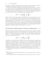
2 Fundamental Concepts of Quantum
Mechanics
2.1 Introduction
Let us start with first discussing the Stern-Gerlach experiment performed in 1922.

Figure 2.1: Diagram of the Stern-Gerlach-Experiment

The magnetic moment of the silver atoms is proportional to the magnetic moment
of the 5s1 electron, the inner electron shells do not have a net magnetic moment. The
Force in z-direction in an inhomogeneous magnetic field is given by
Fz =

∂
∂Bz
µ · B ≈ µz
∂z

∂z

(2.1)

We expect from classical mechanics that the atoms are distributed randomly with a
peak in the middle. But we observe two different peaks; if we calculate the magnetic
moment from the data obtained, we get that the magnetic moment is either S = + /2ez
or S = − /2ez – the electron spin is quantitized.
Historically, more sophisticated experiments followed. Instead of using just one
magnet, several magnets are used in series, so that sequential Stern-Gerlach experiments can be performed:

They show that the spin is quantized in every direction by the amount above, ± /2.
It also suggests that selecting the Sx + component after a Stern-Gerlach experiment
in x-direction completely destroys any previous information about Sz . There is in
fact an analogon in classical mechanics – the transmission of polarized light through
polarization filters.

9

2 Fundamental Concepts of Quantum Mechanics
The following correspondence can be made
Sz ± atoms ↔ x−, y − polarized light
Sx ± atoms ↔ x −, y − polarized light

(2.2)

where x and y -axes are x and y axes rotated by 45◦ .
Notation. We write the Sz+ state as |Sz ; + or |Sz ; ↑ ; similarly, the Sz− state corresponds to |Sz ; ↓ . We assume for Sx states superposition of Sz states
1

? 1
|Sx ; ↑ = √ |Sz ; ↑ + √ |Sz ; ↓
2
2
1
1
?
|Sx ; ↓ = − √ |Sz ; ↑ + √ |Sz ; ↓
2
2

(2.3)
(2.4)

This really is a two-dimensional space! What about the Sy states – it should be a linear
combination of the Sz states, too. However, all possible combinations seem to be used
up. The analogy is circular polarized light. Right circularly polarized light can be
expressed as
i
1
E = E0 √ ex ei(kz−ωt) + √ ey ei(kz−ωt)
2
2

(2.5)

Can we use this analogy to define the Sy states?
i
? 1
|Sx ; ↑ = √ |Sz ; ↑ + √ |Sz ; ↓

2
2
1
i
?
|Sx ; ↓ = − √ |Sz ; ↑ − √ |Sz ; ↓
2
2

(2.6)
(2.7)

We already note here that only the “direction” in the vector space is of significance,
not the “length” of the vectors.

2.2 Kets, Bras, and Operators
Consider a complex vector space of dimension d which is related to the nature of the
physical system.
The space of a single electron spin is two-dimensional whereas for the description
of a free particle a vector space of denumerably infinite dimension is needed.

2.2.1 Kets
The vector space is called Hilbert Space. The physical state is represented by a state
vector. Following Dirac, a state vector is called ket and denoted by |α .
They suffice the usual requirements for vector spaces (commutative, associative addition, existence of null ket and inverse ket, and scalar multiplication).
One important postulate is that |α and c · |α with c = 0 correspond to the same
physical state. Mathematically this means that we deal with rays rather than vectors
A physical observable can be represented by an operator. Operators act on kets from
the left.
A(|α ) = A |α

10

(2.8)

2.2 Kets, Bras, and Operators
In general, applying an operator to a ket cannot be expressed as a scalar multiplication,
i.e.,
A(|α ) = c |α in general

(2.9)

with c any complex number.
Analogously to eigenvectors, there are eigenkets
A(|α ) = a |α , A(|α ) = a |α

,

(2.10)

with eigenvalues a, a , . . ..
Example
Spin 1/2 System. Sz |Sz , ↑ = + 2 |Sz , ↑ , Sz |Sz , ↓ = − 2 |Sz , ↑

The bras belong to the dual vector space.

2.2.2 Bra space and inner product
The Bra space is the vector space dual to the ket space. It is spanned by the eigenbras
{ a |} which correspond to the eigenkets {|a }. There is an isomorphism that assigns

each ket onto its bra.
cα α| + cβ β| ↔ c∗α |α + c∗β |β

α| ↔ |α

(2.11)

Note the complex-conjugated coefficients.
Now we introduce the inner or scalar product1 .
|

:V∗×V ⇒C
( β| , |α ) −→ β|α

(2.12)

It is Hermitian and positive definite, i.e.,
β|α = α|β

∗

α|α ≥ 0 .

(2.13)

Two kets |α and |β are said to be orthogonal if
(2.14)

α|β = 0 .
We can explicitly normalize a ket |˜

α by
|α =

1
α
˜ |˜
α

|˜
α

(2.15)

α
˜ |˜
α is known as the norm of |˜
α.
1 bra)(ket

11

2 Fundamental Concepts of Quantum Mechanics

2.3 Operators
X and Y are said to be equal, X = Y , if X |α = Y |α . Operator addition is commutative and associative,
X + Y = Y + X ; X + (Y + Z) = (X + Y ) + Z .

(2.16)

Operators are usually linear, that is,
X(a1 |α1 + a2 |α2 ) = a1 X |α1 + a2 X |α2

(2.17)

An exception is for example the time-reversal operator which is antilinear.
An operator acts on a bra from the right side.
Note. X |α and α| X are in general not dual to each other. The correspondence is
X |α ↔ α| X †

(2.18)

The operator X † is called the Hermitian adjoint, or simply the adjoint of X. By definition, an operator is said to be Hermitian, if and only if X † = X.

2.3.1 Multiplication of Operators
Multiplication of operators is in general non-commutative, i. e.
XY = Y X

(2.19)

X(Y Z) = (XY )Z

(2.20)

but associative.

Furthermore, the usual rules of a non-Abelian group apply.

2.3.2 Outer Product
The outer product of |β and α| is defined as

(|β )( α|) = |β α|

(2.21)

It is to be regarded as an operator.
|β α| |γ

= |β

ket

(2.22)

α|γ

ket

∈C

Some more rules. Let X be an operator.
|β α|
|β

†

= |α β|

X α| = |β X

β|X|α = α|X † |β

∗
X Hermitian ⇔ β|X|α = α|X|β

12

(2.23)
α| = |β X α|

(2.24)

∗

(2.25)

2.3 Operators

2.3.3 Base Kets and Matrix Representations
Theorem

The eigenvalues of a Hermitian operator A are real; the eigenkets of A
corresponding to different eigenvalues are orthogonal.

Proof
Assume that a is the eigenvalue to the eigenket |α and a is
the eigenvalue to the eigenket |α . Since A is Hermitian, we have a | A = a ∗ a |.
This can be used to obtain
0 = α |A|α − α |A|α
= a α |α − a ∗ α |α = (a − a ∗ ) α |α
This is true if either (for the same state) a = a

same, the eigenkets are orthogonal.

∗

or, if the two eigenvalues are not the

Usually, we will assume that eigenkets are normalized, i. e. αi |αj = δij . Thus, the
eigenkets form an orthogonal set.

2.3.4 Eigenkets as Base Kets
Normalized eigenkets of A form a complete orthonormal set, i. e. an arbitrary ket |β
can be expressed as a linear combination of eigenkets.
|β =

ck |αk

(2.26)

k

If we multiply by αj | we get that αj |β = cj . Thus, we get
|β =

|αk

αk |β

(2.27)

αk | = 1

(2.28)

k

⇒

|αk
k

2.3.5 Resolution of the Identity, Completeness Relation, or Closure
(2.28) can be extremely useful.
β|β = β| 1 |β = β|

|αk

αk | |β

k
2

2

| αk |β | =

=
k

|ck |

..
.

column


...
. . .

..
.

α1 |X|α2
α2 |X|α2
..
.

(2.30)

The Hermitian adjoint of an operator corresponds to the complex conjugate transposed
matrix.
The successive application of operators corresponds to matrix multiplication.
Proof

Let Z = XY .
αi | Z |αj = αi | XY |αj
= αi | X1Y |αj =

αi | X |αk

αk | Y |αj

k

Thus, state kets are represented by column vectors and bras by row vectors.


α1 |β
 α2 |β 


γ| =
ˆ
( γ|α1 , γ|α2 , γ|α3 , . . .)
(2.31)
|β =
ˆ  α3 |β  ,


∗
∗
∗
=
α
|γ
,
α
|γ
,
α

|γ
,
.
.
.
..
1
2
3
.

2.4 Spin 1/2 System
As base kets |Sz ; + = |Sz ; ↑ = |↑ and |Sz ; − = |↓ are used. Since nothing is
special about the z-axis, this just corresponds to a convention. The simplest operators
imaginable is the identity operator 1. In this basis, the operator Sz is diagonal.
1 = |↑ ↑| + |↓ ↓|
Sz =

2

(2.32)

|↑ ↑| − |↓ ↓| =
ˆ

1 0
0 −1

2

(2.33)

Nearly all operators we deal with are Hermitian operators. However, there are some
important non-Hermitian operators, e. g. the so-called lowering and raising operator,
S− and S+ respectively.
S+ = |↑ ↓| =
ˆ

0
0

1
0

(2.34)

S− = |↓ ↑| =
ˆ

0
1

0
0

(2.35)

S± raise and lower the spin by one unit of , respectively. As we will see later, they
can be expressed as
S± = Sx ± iSy

14

(2.36)

2.5 Measurements, Observables And The Uncertainty Relation

2.5 Measurements, Observables And The Uncertainty Relation
Consider a state |α = k ck |αk = k |αk αk |α . According to the quantum theory
of measurement, after a measurement of the observable A the system is ’thrown’ into
an eigenstate of A |αk . We measure A to be αk .
The Result of a measurement yields one of the eigenvalues of A.
Theorem

Postulate
The probability for a state αk to be measured is
2

P (αk ) = | αk |α |

(2.37)

provided that |α normalized.

These probabilities P (αk ) can be determined with a large number of experiments
performed on an ensemble of identically prepared physical systems, a so-called pure
ensemble.
If the system already is in an eigenstate αk , then the probability to measure αk is 1.
The expectation value of an operator A with respect to state α is

A ≡ A

α

≡ α|A|α

(2.38)

This corresponds to the average measured value which can be derived from
A =

α|αj
i,j

αj |A|αi αi |α
=ai δij
2

aj | αj |α | ,

=

(2.39)

j

which corresponds to a sum over the measured values aj which are weighted by the
2
probabilities | αj |α | .
Note. In general, expectation values do not coincide with eigenvalues, e.g. in the

spin 1/2 system, the expectation value is a number that ’arbitrarily’ lies between ± /2.

2.5.1 Compatible Observables
We define the commutator and the anti-commutator as follows:
[A, B] ≡ AB − BA

{A, B} ≡ AB + BA

(2.40)

15

2 Fundamental Concepts of Quantum Mechanics

Definition

Compatible Observables
Observables A and B are defined to be compatible, if the corresponding
operators commute, i. e.
(2.41)

[A, B] = 0
and incompatible, if [A, B] = 0.

If the observables A and B are compatible, then A measurements and B measurements
do not interfere, as we will see below.
An important example for incompatible observables are Sx and Sy , but Sz and S2 ≡
2
k Sk are compatible.

Theorem

Representation of Compatible Observables
Suppose that A and B are compatible observables and the eigenvalues of
A are nondegenerate, i. e. ai = aj ∀i = j, then the matrix elements
αi |B|αj are all diagonal.

Thus, both operators have a common set of eigenkets, their corresponding matrix
representations can be diagonalized simultaneously.
Proof
Simple.
0 = αi |[A, B]|αj = αi |AB − BA|αj
= (αi −
αj∗

) αi |B|αj = 0

(2.42)

=aj Hermitian operator

For different eigenvalues, this means that
αi |B|αj = δij αi |B|αj

16

(2.43)

2.5 Measurements, Observables And The Uncertainty Relation

Assume that A, B, C, . . . with
[A, B] = [A, C] = [B, C] = . . . = 0

(2.46)

form a maximal set of compatible observables which means that we cannot add any
more observables to our list without violating (2.46). Then the (collective) index
Ki = (ai , bi , ci , . . .) uniquely specifies the eigenket
|Ki = |ai , bi , ci , . . .

(2.47)

The completenes relation implies that
|Ki Ki | =

. . . |ai , bi , ci , . . . ai , bi , ci , . . .| = 1
ai

i

bi

|lm lm|

1=
l

(2.48)

ci

(2.49)

|m|≤l

What does it mean when two operators are compatible or not?
Consider a successive measurement of compatible observables.
A

B

A

|α −
→ |ai , bi −
→ |ai , bi −
→ |ai , bi

(2.50)

Thus, A and B measurements do not interfere, if A and B are compatible observables.
Now, imagine an experiment with a sequential selective measurement of incompatible observables.
A

B

C

|α −
→ |ai −

→ |bj −
→ |ck

(2.51)

17

2 Fundamental Concepts of Quantum Mechanics
The probability to find |ck (provided that |ck is normalized) is given by
2

2

P bj (ck ) = | ck |bj | · | bj |ai |

(2.52)

We sum over all bj to get the total probability for going through all possible bj routes.
2

2

| ck |bj | | bj |ai | =

P (ck ) =
j

ck |bj

l

P (ck ) and P (ck ) are different (double sum vs. single sum)! The important result is
that it matters whether or not B is switched on.

2.5.2 Uncertainty Relation
First, we derive the more general uncertainty relation, then – later on – Heisenberg’s
Uncertainty-Relation as a special case of this uncertainty relation.
Given an observable A, we define ∆A as
∆A ≡ A − A

(2.55)

Then we can define the dispersion
∆A

2

=

A2 − 2A A + A

2

= A2 − A

2

(2.56)

which is sometimes also called variance or mean square deviation in accordance with
probabilistic theory.
Remark. Sometimes ∆A denotes
∆A ≡

(∆A)2

(2.57)

Example
2

Theorem

18

(∆Sx )2

Sz ↑

(∆Sz )2

Sz ↑

Uncertainty Relation

=

4
=0

(2.58)
(2.59)

2.5 Measurements, Observables And The Uncertainty Relation

(∆A)2

(∆B)2 ≥

1
2
| [A, B] |
4

(2.60)

If the observables do not commute, then there is some inherent “fuzziness” in the
measurements.
For the proof, we need two lemmas.
Theorem

Schwarz Inequality

2

(2.61)

≥0

(2.62)

α|α β|β ≥ | α|β |

Proof
Note that
α| + λ∗ β| · |α + λ |β
λ can be any complex number. Especially if we set
β|α
β|β
α|β β|α
⇒ α|α −
≥0
β|β
λ := −

(2.63)

This is just equation (2.61).

Theorem
The expectation value of a Hermitian operator is purely real. The expectation value of an anti-Hermitian operator is purely imaginary.

19

Theoretical Physics III Quantum MechanicsAxel Groß23 May 2005

Tài liệu liên quan

Tài liệu bạn tìm kiếm đã sẵn sàng tải về