prandtls essentials of fluid mechanics, herbert oertel

Applied Mathematical Sciences
Volume 158
Editors
S.S. Antman J.E. Marsden L. Sirovich
Advisors
J.K. Hale P. Holmes J. Keener
J. Keller B.J. Matkowsky A. Mielke
C.S. Peskin K.R.S. Sreenivasan


This page intentionally left blank


Herbert Oertel
Editor

Prandtl’s Essentials
of Fluid Mechanics
Second Edition
With Contributions by M. Bo¨hle, D. Etling, U. Mu¨ller,
K.R.S. Sreenivasan, U. Riedel, and J. Warnatz
Translated by Katherine Mayes

With 530 Illustrations


Herbert Oertel
Institut fu¨r Stro¨mungslehre
Universita¨t Karlsruhe
Kaiserstr. 12

Karlsruhe D-76131
Germany

Ludwig Prandtl, em. Prof. Dr. Dr.-Ing. e.h.mult., Universita¨t Go¨ttingen, Dir. MPI fu¨r
Stro¨mungsforschung, † 1953.
Editors:
S.S. Antman
Department of Mathematics
and
Institute for Physical Science
and Technology
University of Maryland
College Park, MD 20742-4015
USA


J.E. Marsden
Control and Dynamical
Systems, 107-81
California Institute of
Technology
Pasadena, CA 91125
USA


L. Sirovich
Division of Applied
Mathematics
Brown University
Providence, RI 02912

USA


Mathematics Subject Classification (2000): 76A02, 76-99
Library of Congress Cataloging-in-Publication Data
Oertel, Herbert.
Prandtl’s essentials of fluid mechanics / Herbert Oertel
p. cm.
Includes bibliographical references and index.
ISBN 0-387-40437-6 (alk. paper)
1. Fluid mechanics. I. Title.
TA357.O33 2003
620.1′06—dc22
2003059136
ISBN 0-387-40437-6

Printed on acid-free paper.

Originally published in the German language by Vieweg Verlag/GWV Fachverlage GmbH, D-65189 Wiesbaden, Germany, as “Herbert Oertel (Hsrg.): Fu¨hrer durch die Stro¨mungslehre. 10. Auflage (10th Edition)”
 Friedr. Vieweg & Sohn Verlagsgesellschaft mbH, Braunschweig/Wiesbaden, 2001.
 2004 Springer-Verlag New York, Inc.
All rights reserved. This work may not be translated or copied in whole or in part without the written
permission of the publisher (Springer-Verlag New York, Inc., 175 Fifth Avenue, New York, NY 10010,
USA), except for brief excerpts in connection with reviews or scholarly analysis. Use in connection
with any form of information storage and retrieval, electronic adaptation, computer software, or by
similar or dissimilar methodology now known or hereafter developed is forbidden.
The use in this publication of trade names, trademarks, service marks, and similar terms, even if they
are not identified as such, is not to be taken as an expression of opinion as to whether or not they are
subject to proprietary rights.
Printed in the United States of America.

9 8 7 6 5 4 3 2 1

(EB)

SPIN 10939734

Springer-Verlag is a part of Springer Science+Business Media
springeronline.com


Preface

Ludwig Prandtl, with his fundamental contributions to hydrodynamics, aerodynamics, and gas dynamics, greatly influenced the development of fluid mechanics as a whole, and it was his pioneering research in the first half of the
last century that founded modern fluid mechanics. His book F¨
uhrer durch
die Str¨
omungslehre, which appeared in 1942, originated from previous publications in 1913, Lehre von der Fl¨
ussigkeit und Gasbewegung, and 1931, Abriß
der Str¨
omungslehre. The title F¨
uhrer durch die Str¨
omungslehre, or Essentials
of Fluid Mechanics, is an indication of Prandtl’s intentions to guide the reader
on a carefully thought-out path through the different areas of fluid mechanics. On his way, the author advances intuitively to the core of the physical
problem, without extensive mathematical derivations. The description of the
fundamental physical phenomena and concepts of fluid mechanics that are
needed to derive the simplified models has priority over a formal treatment
of the methods. This is in keeping with the spirit of Prandtl’s research work.
The first edition of Prandtl’s F¨
uhrer durch die Str¨

omungslehre was the
only book on fluid mechanics of its time and, even today, counts as one of
the most important books in this area. After Prandtl’s death, his students
Klaus Oswatitsch and Karl Wieghardt undertook to continue his work, and to
add new findings in fluid mechanics in the same clear manner of presentation.
When the ninth edition went out of print and a new edition was desired
by the publishers, we were glad to take on the task. The first four chapters of
this book keep to the path marked out by Prandtl in the first edition, in 1942.
The original historical text has been linguistically revised, and leads, after the
Introduction, to chapters on Properties of Liquids and Gases, Kinematics of
Flow, and Dynamics of Fluid Flow. These chapters are taught to science and
engineering students in introductory courses on fluid mechanics even today.
We have retained much of Prandtl’s original material in these chapters, but
added a section on the Topology of a Flow in Chapter 3 and on Flows of NonNewtonian Media in Chapter 4. Chapters 5 and 6, on Fundamental Equations
of Fluid Mechanics and Aerodynamics, enlarges the material in the original,
and forms the basis for the treatment of different branches of fluid mechanics
that appear in subsequent chapters.
The major difference from previous editions lies in the treatment of additional topics of fluid mechanics. The field of fluid mechanics is continuously


VI

Preface

growing, and has now become so extensive that a selection had to be made.
I am greatly indebted to my colleagues K.R. Sreenivasan, U. M¨
uller, J. Warnatz, U. Riedel, D. Etling, and M. B¨ohle, who revised individual chapters in
their own research areas, keeping Prandtl’s purpose in mind and presenting
the latest developments of the last sixty years in Chapters 7 to 14. Some of
these chapters can be found in some form in Prandtl’s book, but have undergone substantial revisions; others are entirely new. The original chapters

on Wing Aerodynamics, Heat Transfer, Stratified Flows, Turbulent Flows,
Multiphase Flows, Flows in the Atmosphere and the Ocean, and Thermal
Turbomachinery have been revised, while the chapters on Fluid Mechanical
Instabilities, Flows with Chemical Reactions, and Biofluid Mechanics of Blood
Circulation are new. References to the literature in the individual chapters
have intentionally been kept to those few necessary for comprehension and
completion. The extensive historical citations may be found by referring to
previous editions.
Essentials of Fluid Mechanics is targeted to science and engineering students who, having had some basic exposure to fluid mechanics, wish to attain
an overview of the different branches of fluid mechanics. The presentation
postpones the use of vectors and eschews the use integral theorems in order
to preserve the accessibility to this audience. For more general and compact
mathematical derivations we refer to the references. In order to give students
the possibility of checking their learning of the subject matter, Chapters 2
to 6 are supplemented with problems. The book will also give the expert in
research or industry valuable stimulation in the treatment and solution of
fluid-mechanical problems.
We hope that we have been able, with the treatment of the different
branches of fluid mechanics, to carry on the work of Ludwig Prandtl as he
would have wished. Chapters 1–6, 8, 9, and 13 were written by H. Oertel
Jr., Chapter 7 by K.R. Sreenivasan, Chapter 10 by U. M¨
uller, Chapter 11 by
J. Warnatz and U. Riedel, Chapter 12 by D. Etling, and Chapter 14 by M.
B¨
ohle. Thanks are due to those colleagues whose numerous suggestions have
been included in the text.
I thank Katherine Mayes for the translation and typesetting of the English manuscript and U. Dohrmann for the completion of the text files. The
extremely fruitful collaboration with Springer-Verlag also merits particular
praise.
Karlsruhe, June 2003

Herbert Oertel


Contents

Preface . . . . . . . . . . . . . . . . . . . . . . . . . . . . . . . . . . . . . . . . . . . . . . . . . . . . . . .

V

1.

Introduction . . . . . . . . . . . . . . . . . . . . . . . . . . . . . . . . . . . . . . . . . . . . . .

1

2.

Properties of Liquids and Gases . . . . . . . . . . . . . . . . . . . . . . . . . .
2.1 Properties of Liquids . . . . . . . . . . . . . . . . . . . . . . . . . . . . . . . . . . . .
2.2 State of Stress . . . . . . . . . . . . . . . . . . . . . . . . . . . . . . . . . . . . . . . . .
2.3 Liquid Pressure . . . . . . . . . . . . . . . . . . . . . . . . . . . . . . . . . . . . . . . .
2.4 Properties of Gases . . . . . . . . . . . . . . . . . . . . . . . . . . . . . . . . . . . . .
2.5 Gas Pressure . . . . . . . . . . . . . . . . . . . . . . . . . . . . . . . . . . . . . . . . . . .
2.6 Interaction Between Gas Pressure and Liquid Pressure . . . . . .
2.7 Equilibrium in Other Force Fields . . . . . . . . . . . . . . . . . . . . . . . .
2.8 Surface Stress (Capillarity) . . . . . . . . . . . . . . . . . . . . . . . . . . . . . .
2.9 Problems . . . . . . . . . . . . . . . . . . . . . . . . . . . . . . . . . . . . . . . . . . . . . .

17

17
18
21
26
29
32
35
39
42

3.

Kinematics of Fluid Flow . . . . . . . . . . . . . . . . . . . . . . . . . . . . . . . . .
3.1 Methods of Representation . . . . . . . . . . . . . . . . . . . . . . . . . . . . . .
3.2 Acceleration of a Flow . . . . . . . . . . . . . . . . . . . . . . . . . . . . . . . . . .
3.3 Topology of a Flow . . . . . . . . . . . . . . . . . . . . . . . . . . . . . . . . . . . . .
3.4 Problems . . . . . . . . . . . . . . . . . . . . . . . . . . . . . . . . . . . . . . . . . . . . . .

47
47
51
52
59

4.

Dynamics of Fluid Flow . . . . . . . . . . . . . . . . . . . . . . . . . . . . . . . . . .
4.1 Dynamics of Inviscid Liquids . . . . . . . . . . . . . . . . . . . . . . . . . . . . .
4.1.1 Continuity and the Bernoulli Equation . . . . . . . . . . . . . .
4.1.2 Consequences of the Bernoulli Equation . . . . . . . . . . . . .

4.1.3 Pressure Measurement . . . . . . . . . . . . . . . . . . . . . . . . . . . .
4.1.4 Interfaces and Formation of Vortices . . . . . . . . . . . . . . . .
4.1.5 Potential Flow . . . . . . . . . . . . . . . . . . . . . . . . . . . . . . . . . . .
4.1.6 Wing Lift and the Magnus Effect . . . . . . . . . . . . . . . . . . .
4.1.7 Balance of Momentum for Steady Flows . . . . . . . . . . . . .
4.1.8 Waves on a Free Liquid Surface . . . . . . . . . . . . . . . . . . . .
4.1.9 Problems . . . . . . . . . . . . . . . . . . . . . . . . . . . . . . . . . . . . . . . .
4.2 Dynamics of Viscous Liquids . . . . . . . . . . . . . . . . . . . . . . . . . . . . .
4.2.1 Viscosity (Inner Friction), the Navier–Stokes Equation

63
63
63
67
75
77
80
93
95
103
113
118
118


VIII

Contents

4.2.2 Mechanical Similarity, Reynolds Number . . . . . . . . . . . .

4.2.3 Laminar Boundary Layers . . . . . . . . . . . . . . . . . . . . . . . . .
4.2.4 Onset of Turbulence . . . . . . . . . . . . . . . . . . . . . . . . . . . . . .
4.2.5 Fully Developed Turbulence . . . . . . . . . . . . . . . . . . . . . . .
4.2.6 Flow Separation and Vortex Formation . . . . . . . . . . . . . .
4.2.7 Secondary Flows . . . . . . . . . . . . . . . . . . . . . . . . . . . . . . . . .
4.2.8 Flows with Prevailing Viscosity . . . . . . . . . . . . . . . . . . . .
4.2.9 Flows Through Pipes and Channels . . . . . . . . . . . . . . . . .
4.2.10 Drag of Bodies in Liquids . . . . . . . . . . . . . . . . . . . . . . . . .
4.2.11 Flows in Non-Newtonian Media . . . . . . . . . . . . . . . . . . . .
4.2.12 Problems . . . . . . . . . . . . . . . . . . . . . . . . . . . . . . . . . . . . . . . .
4.3 Dynamics of Gases . . . . . . . . . . . . . . . . . . . . . . . . . . . . . . . . . . . . .
4.3.1 Pressure Propagation, Velocity of Sound . . . . . . . . . . . .
4.3.2 Steady Compressible Flows . . . . . . . . . . . . . . . . . . . . . . . .
4.3.3 Conservation of Energy . . . . . . . . . . . . . . . . . . . . . . . . . . .
4.3.4 Theory of Normal Shock Waves . . . . . . . . . . . . . . . . . . . .
4.3.5 Flows past Corners, Free Jets . . . . . . . . . . . . . . . . . . . . . .
4.3.6 Flows with Small Perturbations . . . . . . . . . . . . . . . . . . . .
4.3.7 Flows past Airfoils . . . . . . . . . . . . . . . . . . . . . . . . . . . . . . .
4.3.8 Problems . . . . . . . . . . . . . . . . . . . . . . . . . . . . . . . . . . . . . . . .

122
123
126
136
144
151
153
160
165
175

180
186
186
190
195
196
200
203
207
213

5.

Fundamental Equations of Fluid Mechanics . . . . . . . . . . . . . . .
5.1 Continuity Equation . . . . . . . . . . . . . . . . . . . . . . . . . . . . . . . . . . . .
5.2 Navier–Stokes Equations . . . . . . . . . . . . . . . . . . . . . . . . . . . . . . . .
5.2.1 Laminar Flows . . . . . . . . . . . . . . . . . . . . . . . . . . . . . . . . . . .
5.2.2 Reynolds Equations for Turbulent Flows . . . . . . . . . . . .
5.3 Energy Equation . . . . . . . . . . . . . . . . . . . . . . . . . . . . . . . . . . . . . . .
5.3.1 Laminar Flows . . . . . . . . . . . . . . . . . . . . . . . . . . . . . . . . . . .
5.3.2 Turbulent Flows . . . . . . . . . . . . . . . . . . . . . . . . . . . . . . . . . .
5.4 Fundamental Equations as Conservation Laws . . . . . . . . . . . . . .
5.4.1 Hierarchy of Fundamental Equations . . . . . . . . . . . . . . . .
5.4.2 Navier–Stokes Equations . . . . . . . . . . . . . . . . . . . . . . . . . .
5.4.3 Derived Model Equations . . . . . . . . . . . . . . . . . . . . . . . . . .
5.4.4 Reynolds Equations for Turbulent Flows . . . . . . . . . . . .
5.4.5 Multiphase Flows . . . . . . . . . . . . . . . . . . . . . . . . . . . . . . . .
5.4.6 Reactive Flows . . . . . . . . . . . . . . . . . . . . . . . . . . . . . . . . . . .
5.5 Differential Equations of Perturbations . . . . . . . . . . . . . . . . . . . .
5.6 Problems . . . . . . . . . . . . . . . . . . . . . . . . . . . . . . . . . . . . . . . . . . . . . .

217
217
218
218
225
230
230
234
236
236
237
240
247
248
251
253
258

6.

Aerodynamics . . . . . . . . . . . . . . . . . . . . . . . . . . . . . . . . . . . . . . . . . . . .
6.1 Fundamentals of Aerodynamics . . . . . . . . . . . . . . . . . . . . . . . . . .
6.1.1 Bird Flight and Technical Imitations . . . . . . . . . . . . . . .
6.1.2 Airfoils and Wings . . . . . . . . . . . . . . . . . . . . . . . . . . . . . . .
6.1.3 Airfoil and Wing Theory . . . . . . . . . . . . . . . . . . . . . . . . . .
6.1.4 Aerodynamic Facilities . . . . . . . . . . . . . . . . . . . . . . . . . . .

265
265

266
268
276
290


Contents

7.

8.

IX

6.2 Transonic Aerodynamics . . . . . . . . . . . . . . . . . . . . . . . . . . . . . . . .
6.2.1 Swept Wings . . . . . . . . . . . . . . . . . . . . . . . . . . . . . . . . . . . .
6.2.2 Shock–Boundary-Layer Interaction . . . . . . . . . . . . . . . . .
6.2.3 Flow Separation . . . . . . . . . . . . . . . . . . . . . . . . . . . . . . . . . .
6.3 Supersonic Aerodynamics . . . . . . . . . . . . . . . . . . . . . . . . . . . . . . . .
6.3.1 Delta Wings . . . . . . . . . . . . . . . . . . . . . . . . . . . . . . . . . . . . .
6.4 Problems . . . . . . . . . . . . . . . . . . . . . . . . . . . . . . . . . . . . . . . . . . . . . .

292
294
297
304
306
307
314

Turbulent Flows . . . . . . . . . . . . . . . . . . . . . . . . . . . . . . . . . . . . . . . . . .
7.1 Fundamentals of Turbulent Flows . . . . . . . . . . . . . . . . . . . . . . . .
7.2 Onset of Turbulence . . . . . . . . . . . . . . . . . . . . . . . . . . . . . . . . . . . .
7.2.1 Linear Stability . . . . . . . . . . . . . . . . . . . . . . . . . . . . . . . . . .
7.2.2 Nonlinear Stability . . . . . . . . . . . . . . . . . . . . . . . . . . . . . . .
7.2.3 Nonnormal Stability . . . . . . . . . . . . . . . . . . . . . . . . . . . . . .
7.3 Developed Turbulence . . . . . . . . . . . . . . . . . . . . . . . . . . . . . . . . . . .
7.3.1 The Notion of a Mixing Length . . . . . . . . . . . . . . . . . . . .
7.3.2 Turbulent Mixing . . . . . . . . . . . . . . . . . . . . . . . . . . . . . . . .
7.3.3 Energy Relations in Turbulent Flows . . . . . . . . . . . . . . . .
7.4 Classes of Turbulent Flows . . . . . . . . . . . . . . . . . . . . . . . . . . . . . .
7.4.1 Free Turbulence . . . . . . . . . . . . . . . . . . . . . . . . . . . . . . . . . .
7.4.2 Flow Along a Boundary . . . . . . . . . . . . . . . . . . . . . . . . . . .
7.4.3 Rotating and Stratified Flows, Flows with Curvature
Effects . . . . . . . . . . . . . . . . . . . . . . . . . . . . . . . . . . . . . . . . . .
7.4.4 Turbulence in Tunnels . . . . . . . . . . . . . . . . . . . . . . . . . . . .
7.4.5 Two-Dimensional Turbulence . . . . . . . . . . . . . . . . . . . . . .
7.5 New Developments in Turbulence . . . . . . . . . . . . . . . . . . . . . . . . .
7.5.1 Lagrangian Investigations of Turbulence . . . . . . . . . . . . .
7.5.2 Field-Theoretic Methods . . . . . . . . . . . . . . . . . . . . . . . . . .
7.5.3 Outlook . . . . . . . . . . . . . . . . . . . . . . . . . . . . . . . . . . . . . . . . .

319
319
320
321
323
324
326
326

328
329
331
331
334
337
340
344
348
353
354
354

Fluid-Mechanical Instabilities . . . . . . . . . . . . . . . . . . . . . . . . . . . . .
8.1 Fundamentals of Fluid-Mechanical Instabilities . . . . . . . . . . . . .
8.1.1 Examples of Fluid-Mechanical Instabilities . . . . . . . . . . .
8.1.2 Definition of Stability . . . . . . . . . . . . . . . . . . . . . . . . . . . . .
8.1.3 Local Perturbations . . . . . . . . . . . . . . . . . . . . . . . . . . . . . .
8.2 Stratification Instabilities . . . . . . . . . . . . . . . . . . . . . . . . . . . . . . . .
8.2.1 Rayleigh–B´enard Convection . . . . . . . . . . . . . . . . . . . . . . .
8.2.2 Marangoni Convection . . . . . . . . . . . . . . . . . . . . . . . . . . . .
8.2.3 Diffusion Convection . . . . . . . . . . . . . . . . . . . . . . . . . . . . . .
8.3 Hydrodynamic Instabilities . . . . . . . . . . . . . . . . . . . . . . . . . . . . . .
8.3.1 Taylor Instability . . . . . . . . . . . . . . . . . . . . . . . . . . . . . . . . .
8.3.2 G¨ortler Instability . . . . . . . . . . . . . . . . . . . . . . . . . . . . . . . .
8.4 Shear-Flow Instabilities . . . . . . . . . . . . . . . . . . . . . . . . . . . . . . . . .
8.4.1 Boundary-Layer Flows . . . . . . . . . . . . . . . . . . . . . . . . . . . .
8.4.2 Tollmien–Schlichting and Cross-Flow Instabilities . . . . .

357

357
357
363
366
367
367
379
382
388
388
393
395
396
403


X

Contents

8.4.3 Kelvin–Helmholtz Instability . . . . . . . . . . . . . . . . . . . . . . . 419
8.4.4 Wake Flows . . . . . . . . . . . . . . . . . . . . . . . . . . . . . . . . . . . . . 422
9.

Convective Heat and Mass Transfer . . . . . . . . . . . . . . . . . . . . . .
9.1 Fundamentals of Heat and Mass Transfer . . . . . . . . . . . . . . . . . .
9.1.1 Free and Forced Convection . . . . . . . . . . . . . . . . . . . . . . .
9.1.2 Heat Conduction and Convection . . . . . . . . . . . . . . . . . . .
9.1.3 Diffusion and Convection . . . . . . . . . . . . . . . . . . . . . . . . . .
9.2 Free Convection . . . . . . . . . . . . . . . . . . . . . . . . . . . . . . . . . . . . . . . .

9.2.1 Convection at a Vertical Plate . . . . . . . . . . . . . . . . . . . . .
9.2.2 Convection at a Horizontal Cylinder . . . . . . . . . . . . . . . .
9.3 Forced Convection . . . . . . . . . . . . . . . . . . . . . . . . . . . . . . . . . . . . . .
9.3.1 Pipe Flows . . . . . . . . . . . . . . . . . . . . . . . . . . . . . . . . . . . . . .
9.3.2 Boundary-Layer Flows . . . . . . . . . . . . . . . . . . . . . . . . . . . .
9.3.3 Bodies in Flows . . . . . . . . . . . . . . . . . . . . . . . . . . . . . . . . . .
9.4 Heat and Mass Exchange . . . . . . . . . . . . . . . . . . . . . . . . . . . . . . . .
9.4.1 Mass Exchange at the Flat Plate . . . . . . . . . . . . . . . . . . .

427
427
427
429
430
431
431
437
438
438
442
449
449
450

10. Multiphase Flows . . . . . . . . . . . . . . . . . . . . . . . . . . . . . . . . . . . . . . . . .
10.1 Fundamentals of Multiphase Flows . . . . . . . . . . . . . . . . . . . . . . .
10.1.1 Definitions . . . . . . . . . . . . . . . . . . . . . . . . . . . . . . . . . . . . . .
10.1.2 Flow Patterns . . . . . . . . . . . . . . . . . . . . . . . . . . . . . . . . . . . .
10.1.3 Flow Pattern Maps . . . . . . . . . . . . . . . . . . . . . . . . . . . . . . .
10.2 Flow Models . . . . . . . . . . . . . . . . . . . . . . . . . . . . . . . . . . . . . . . . . . .

10.2.1 The One-Dimensional Two-Fluid Model . . . . . . . . . . . . .
10.2.2 Mixing Models . . . . . . . . . . . . . . . . . . . . . . . . . . . . . . . . . . .
10.2.3 The Drift–Flow Model . . . . . . . . . . . . . . . . . . . . . . . . . . . .
10.2.4 Bubbles and Drops . . . . . . . . . . . . . . . . . . . . . . . . . . . . . . .
10.2.5 Spray Flows . . . . . . . . . . . . . . . . . . . . . . . . . . . . . . . . . . . . .
10.3 Pressure Loss and Volume Fraction in Hydraulic Components
10.3.1 Friction Loss in Horizontal Straight Pipes . . . . . . . . . . .
10.3.2 Acceleration Losses . . . . . . . . . . . . . . . . . . . . . . . . . . . . . . .
10.4 Propagation Velocity of Density Waves and Critical Mass
Fluxes . . . . . . . . . . . . . . . . . . . . . . . . . . . . . . . . . . . . . . . . . . . . . . . .
10.4.1 Density Waves . . . . . . . . . . . . . . . . . . . . . . . . . . . . . . . . . . .
10.4.2 Critical Mass Fluxes . . . . . . . . . . . . . . . . . . . . . . . . . . . . . .
10.4.3 Cavitation . . . . . . . . . . . . . . . . . . . . . . . . . . . . . . . . . . . . . . .
10.5 Instabilities in Two-Phase Flows . . . . . . . . . . . . . . . . . . . . . . . . .

453
453
454
457
457
460
461
464
466
468
471
474
475
479

11. Reactive Flows . . . . . . . . . . . . . . . . . . . . . . . . . . . . . . . . . . . . . . . . . . .
11.1 Fundamentals of Reactive Flows . . . . . . . . . . . . . . . . . . . . . . . . . .
11.1.1 Rate Laws and Reaction Orders . . . . . . . . . . . . . . . . . . . .
11.1.2 Relation Between Forward and Reverse Reactions . . . .
11.1.3 Elementary Reactions and Reaction Molecularity . . . . .
11.1.4 Temperature Dependence of Rate Coefficients . . . . . . . .

503
503
503
504
505
508

483
483
486
493
497


Contents

XI

11.1.5 Pressure Dependence of Rate Coefficients . . . . . . . . . . . .
11.1.6 Characteristics of Reaction Mechanisms . . . . . . . . . . . . .
11.2 Laminar Reactive Flows . . . . . . . . . . . . . . . . . . . . . . . . . . . . . . . . .
11.2.1 Structure of Premixed Flames . . . . . . . . . . . . . . . . . . . . . .
11.2.2 Flame Velocity of Premixed Flames . . . . . . . . . . . . . . . . .

11.2.3 Sensitivity Analysis . . . . . . . . . . . . . . . . . . . . . . . . . . . . . . .
11.2.4 Nonpremixed Counterflow Flames . . . . . . . . . . . . . . . . . .
11.2.5 Nonpremixed Jet Flames . . . . . . . . . . . . . . . . . . . . . . . . . .
11.2.6 Nonpremixed Flames with Fast Chemistry . . . . . . . . . . .
11.2.7 Exhaust Gas Cleaning with Plasma Sources . . . . . . . . . .
11.2.8 Flows in Etching Reactors . . . . . . . . . . . . . . . . . . . . . . . . .
11.2.9 Heterogeneous Catalysis . . . . . . . . . . . . . . . . . . . . . . . . . . .
11.3 Turbulent Reactive Flows . . . . . . . . . . . . . . . . . . . . . . . . . . . . . . .
11.3.1 Overview and Concepts . . . . . . . . . . . . . . . . . . . . . . . . . . .
11.3.2 Direct Numerical Simulation . . . . . . . . . . . . . . . . . . . . . . .
11.3.3 Turbulence Models . . . . . . . . . . . . . . . . . . . . . . . . . . . . . . .
11.3.4 Mean Reaction Rates . . . . . . . . . . . . . . . . . . . . . . . . . . . . .
11.3.5 Eddy-Break-Up Models . . . . . . . . . . . . . . . . . . . . . . . . . . .
11.3.6 Large-Eddy Simulation (LES) . . . . . . . . . . . . . . . . . . . . . .
11.3.7 Turbulent Nonpremixed Flames . . . . . . . . . . . . . . . . . . . .
11.3.8 Turbulent Premixed Flames . . . . . . . . . . . . . . . . . . . . . . .
11.4 Hypersonic Flows . . . . . . . . . . . . . . . . . . . . . . . . . . . . . . . . . . . . . . .
11.4.1 Physical-Chemical Phenomena in Reentry Flight . . . . .
11.4.2 Chemical Nonequilibrium . . . . . . . . . . . . . . . . . . . . . . . . . .
11.4.3 Thermal Nonequilibrium . . . . . . . . . . . . . . . . . . . . . . . . . .
11.4.4 Surface Reactions on Reentry Vehicles . . . . . . . . . . . . . .

510
512
517
517
520
521
523
525

526
527
530
531
532
532
533
535
536
542
542
543
554
560
560
561
564
567

12. Flows in the Atmosphere and in the Ocean . . . . . . . . . . . . . . .
12.1 Fundamentals of Flows in the Atmosphere and in the Ocean .
12.1.1 Introduction . . . . . . . . . . . . . . . . . . . . . . . . . . . . . . . . . . . . .
12.1.2 Fundamental Equations in Rotating Systems . . . . . . . . .
12.1.3 Geostrophic Flow . . . . . . . . . . . . . . . . . . . . . . . . . . . . . . . . .
12.1.4 Vorticity . . . . . . . . . . . . . . . . . . . . . . . . . . . . . . . . . . . . . . . .
12.1.5 Ekman Layer . . . . . . . . . . . . . . . . . . . . . . . . . . . . . . . . . . . .
12.1.6 Prandtl Layer . . . . . . . . . . . . . . . . . . . . . . . . . . . . . . . . . . . .
12.2 Flows in the Atmosphere . . . . . . . . . . . . . . . . . . . . . . . . . . . . . . . .
12.2.1 Thermal Wind Systems . . . . . . . . . . . . . . . . . . . . . . . . . . .
12.2.2 Thermal Convection . . . . . . . . . . . . . . . . . . . . . . . . . . . . . .

12.2.3 Gravity Waves . . . . . . . . . . . . . . . . . . . . . . . . . . . . . . . . . . .
12.2.4 Vortices . . . . . . . . . . . . . . . . . . . . . . . . . . . . . . . . . . . . . . . . .
12.2.5 Global Atmospheric Circulation . . . . . . . . . . . . . . . . . . . .
12.3 Flows in the Ocean . . . . . . . . . . . . . . . . . . . . . . . . . . . . . . . . . . . . .
12.3.1 Wind-Driven Flows . . . . . . . . . . . . . . . . . . . . . . . . . . . . . . .
12.3.2 Water Waves . . . . . . . . . . . . . . . . . . . . . . . . . . . . . . . . . . . .
12.4 Application to Atmospheric and Oceanic Flows . . . . . . . . . . . . .

571
571
571
571
574
576
579
582
584
584
588
590
592
598
600
601
603
606


XII

Contents

12.4.1 Weather Forecast . . . . . . . . . . . . . . . . . . . . . . . . . . . . . . . . . 606
12.4.2 Greenhouse Effect and Climate Prediction . . . . . . . . . . . 608
12.4.3 Ozone Hole . . . . . . . . . . . . . . . . . . . . . . . . . . . . . . . . . . . . . . 612
13. Biofluid Mechanics of Blood Circulation . . . . . . . . . . . . . . . . . .
13.1 Fundamentals of Biofluid Mechanics . . . . . . . . . . . . . . . . . . . . . .
13.1.1 Respiratory System . . . . . . . . . . . . . . . . . . . . . . . . . . . . . . .
13.1.2 Blood Circulation . . . . . . . . . . . . . . . . . . . . . . . . . . . . . . . .
13.1.3 Rheology of the Blood . . . . . . . . . . . . . . . . . . . . . . . . . . . .
13.2 Flow in the Heart . . . . . . . . . . . . . . . . . . . . . . . . . . . . . . . . . . . . . .
13.2.1 Physiology and Anatomy of the Heart . . . . . . . . . . . . . . .
13.2.2 Structure of the Heart . . . . . . . . . . . . . . . . . . . . . . . . . . . .
13.2.3 Excitation Physiology of the Heart . . . . . . . . . . . . . . . . .
13.2.4 Flow in the Heart . . . . . . . . . . . . . . . . . . . . . . . . . . . . . . . .
13.2.5 Cardiac Valves . . . . . . . . . . . . . . . . . . . . . . . . . . . . . . . . . . .
13.3 Flow in Blood Vessels . . . . . . . . . . . . . . . . . . . . . . . . . . . . . . . . . . .
13.3.1 Unsteady Pipe Flow . . . . . . . . . . . . . . . . . . . . . . . . . . . . . .
13.3.2 Unsteady Arterial Flow . . . . . . . . . . . . . . . . . . . . . . . . . . .
13.3.3 Arterial Branches . . . . . . . . . . . . . . . . . . . . . . . . . . . . . . . .

615
615
618
620
625
626
627
630
634

637
642
645
649
650
653

14. Thermal Turbomachinery . . . . . . . . . . . . . . . . . . . . . . . . . . . . . . . . .
14.1 Fundamentals of Thermal Turbomachinery . . . . . . . . . . . . . . . .
14.2 Axial Compressor . . . . . . . . . . . . . . . . . . . . . . . . . . . . . . . . . . . . . .
14.2.1 Flow Coefficient, Pressure Coefficient, and Degree of
Reaction . . . . . . . . . . . . . . . . . . . . . . . . . . . . . . . . . . . . . . . .
14.2.2 Method of Design . . . . . . . . . . . . . . . . . . . . . . . . . . . . . . . .
14.2.3 Subsonic Compressor . . . . . . . . . . . . . . . . . . . . . . . . . . . . .
14.2.4 Transonic Compressor . . . . . . . . . . . . . . . . . . . . . . . . . . . .
14.3 Centrifugal Compressor . . . . . . . . . . . . . . . . . . . . . . . . . . . . . . . . .
14.3.1 Flow Physics of the Centrifugal Compressor . . . . . . . . .
14.3.2 Flow Coefficient, Pressure Coefficient, and Efficiency . .
14.3.3 Slip Factor . . . . . . . . . . . . . . . . . . . . . . . . . . . . . . . . . . . . . .
14.4 Combustion Chamber . . . . . . . . . . . . . . . . . . . . . . . . . . . . . . . . . . .
14.4.1 Flow with Heat Transfer . . . . . . . . . . . . . . . . . . . . . . . . . .
14.4.2 Geometry of the Combustion Chamber . . . . . . . . . . . . . .
14.5 Turbine . . . . . . . . . . . . . . . . . . . . . . . . . . . . . . . . . . . . . . . . . . . . . . .
14.5.1 Basics . . . . . . . . . . . . . . . . . . . . . . . . . . . . . . . . . . . . . . . . . .
14.5.2 Efficiency, Flow Coefficient, Work Coefficient, and
Degree of Reaction . . . . . . . . . . . . . . . . . . . . . . . . . . . . . . .
14.5.3 Impulse and Reaction Stage . . . . . . . . . . . . . . . . . . . . . . .

655
655

659
659
663
666
668
672
672
676
678
679
679
681
682
682
683
684

Selected Bibliography . . . . . . . . . . . . . . . . . . . . . . . . . . . . . . . . . . . . . . . . . 687
Index . . . . . . . . . . . . . . . . . . . . . . . . . . . . . . . . . . . . . . . . . . . . . . . . . . . . . . . . . 715


1. Introduction

The development of modern fluid mechanics is closely connected to the name
of its founder, Ludwig Prandtl. In 1904 it was his famous article on fluid
motion with very small friction that introduced boundary-layer theory. His
article on airfoil theory, published the following decade, formed the basis
for the calculation of friction drag, heat transfer, and flow separation. He
introduced fundamental ideas on the modeling of turbulent flows with the
Prandtl mixing length for turbulent momentum exchange. His work on gas

dynamics, such as the Prandtl–Glauert correction for compressible flows, the
theory of shock waves and expansion waves, as well as the first photographs
of supersonic flows in nozzles, reshaped this research area. He applied the
methods of fluid mechanics to meteorology, and was also pioneering in his
contributions to problems of elasticity, plasticity, and rheology.
Prandtl was particularly successful in bringing together theory and experiment, with the experiments serving to verify his theoretical ideas. It was this
that gave Prandtl’s experiments their importance and precision. His famous
experiment with the tripwire, through which he discovered the turbulent
boundary layer and the effect of turbulence on flow separation, is one example. The tripwire was not merely inspiration, but rather was the result of
consideration of discrepancies in Eiffel’s drag measurements on spheres. Two
experiments with different tripwire positions were enough to establish the
generation of turbulence and its effect on the flow separation. For his experiments Prandtl developed wind tunnels and measuring apparatus, such as the
G¨ottingen wind tunnel and the Prandtl stagnation tube. His scientific results
often seem to be intuitive, with the mathematical derivation present only to
provide service to the physical understanding, although it then does indeed
deliver the decisive result and the simplified physical model. According to a
comment by Werner Heisenberg, Prandtl was able to “see” the solutions of
differential equations without calculating them.
Selected individual examples aim to introduce the reader to the path to
understanding of fluid mechanics prepared by Prandtl and to the contents and
modeling in each chapter. As an example of the dynamics of flows, the different regimes in the flow past a vehicle, an incompressible flow (hydrodynamics,
Chapter 4), and in the flow past a wing, a compressible flow (aerodynamics,
Chapter 6) are described.


2

1. Introduction

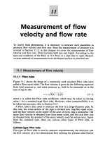
In the flow past a vehicle, we differentiate between the free flow past the

surface and the flow between the vehicle moving with velocity u∞ and the
street at rest. At the stagnation point, where the pressure is at its maximum,
the flow divides, and is accelerated along the hood and past the spoiler along
the base of the vehicle. This leads to a pressure drop and to a negative
downward pressure to the street, as shown in Figure 1.1. The flow again
slows down at the windshield, and is decelerated downstream along the roof
and the trunk. This leads to a pressure increase with a positive lift, while the
negative downward pressure on the street along the lower side of the vehicle
remains.
The viscous flow (Section 4.2) on the upper and lower sides of the vehicle
is restricted to the boundary-layer flow, which passes over to the viscous wake
at the back edge of the vehicle. The flow in the wind tunnel experiment is
made visible with smoke, and this shows that downstream from the back of
the automobile, a backflow region forms. This is seen in the figure as the
black region. Outside the boundary layer and the wake, the flow is essentially
inviscid (Section 4.1).
In order to be able to understand the different flow regimes, and therefore
to establish a basis for the aerodynamic design of a motor vehicle, Prandtl
worked out the carefully prepared path (Chapters 2 to 4) from the properties
of liquids and gases, to kinematics, and to the dynamics of inviscid and viscous
flows. By following this path, too, the reader will successively gain physical
understanding of this first flow example.
The second flow example considers the compressible flow past a wing with
a shock wave (Sections 4.3 and 6.2). The free flow toward the wing has the
velocity of a civil aircraft u∞ , a large subsonic velocity. Figure 1.2 shows
reibungsfreie
inviscid flow Umströmung

8

uu

Grenzschicht
boundary layer
Nachlauf
wake

-

+

+

-

+
-

-

Fig. 1.1. Flow past a vehicle

wake flow visualization


1. Introduction

3

the flow regimes on a cross-section of the wing and the negative pressure

distribution, with the flow again made visible with small particles. From the
stagnation point, the stagnation line bifurcates to follow the suction side (upper side) and the pressure side (lower side) of the wing. On the upper side,
the flow is accelerated up to supersonic velocities, an effect that is connected
with a large pressure drop. Further downstream, the flow is again decelerated
to the subsonic regime via a compression shock wave. This shock wave interacts with the boundary layer and causes it to thicken, leading to increased
drag.
On the lower side the flow is also accelerated from the stagnation point.
However, the acceleration in the nose region is not as great as that on the
suction side, and so no supersonic velocities occur along the pressure side.
From about the middle of the wing onwards, the flow is again decelerated.
The pressures above and below then approach one another, leading to the
wake region downstream of the trailing edge.
A thin boundary layer is formed on the suction and pressure sides of the
wing. The suction and pressure side boundary layers meet at the trailing edge
and form the wake flow downstream. As in the example of the flow past a
motor vehicle, both the flow in the boundary layers and the flow in the wake
are viscous. Outside these regions the flow is essentially inviscid.
The pressure distribution in Figure 1.2 results in a lift, which, for the
wing of the civil aircraft, has to be adapted to the number of passengers to
be transported. In designing the wing, the design engineer has to keep the
drag of the wing as small as possible to save fuel. This is done by shaping
the wing appropriately.
inviscid flow Umströmung
reibungsfreie
Stoss
shock

Grenzschicht
boundary
layer

8

uu

wake
Nachlauf

-c
− pcp
+
+

x

-1
−1

Fig. 1.2. Flow past a wing

flow visualization


4

1. Introduction

Different equations for computing each flow result from the different properties of each flow regime. To good approximation, the boundary-layer equations hold in the boundary-layer regime. In contrast, computing the wake
flow and the flow close to the trailing edge is more difficult. In these regimes,
the Navier–Stokes equations have to be solved. The inviscid flow in the region in front of the shock can be treated using the potential equation, a

comparatively simple task. The inviscid flow behind the shock outside the
boundary layer has to be computed with the Euler equations, since the flow
there is rotational. In the shock-boundary-layer interaction region, again the
Navier–Stokes equations have to be solved.
In contrast to Prandtl’s day, numerical software is now available for solving the different partial differential equations. Because of this, in Chapter
5 we present the fundamental equations of laminar and turbulent flows as a
basis for the following chapters dealing with the different branches of fluid
mechanics. Following the same procedure as Prandtl, the mathematical solution algorithms and methods are to be found by referral to the texts and
literature cited.
As will be shown in Chapters 6 to 14, in spite of numerically computed
flow fields, it is necessary to consider the physical modeling in the different
regimes. There are still no closed theories of turbulent flows, of multiphase
flows, or of the coupling of flows with chemical reactions out of thermal
or chemical equilibrium. For this reason, Prandtl’s method of intuitive connection of theory and experiment to physical modeling is still very much
up-to-date.
The fascinating complexity of turbulence has attracted the attention of
scientists for centuries (Chapter 7). For example, the swirling motion of fluids
that occurs irregularly in space and time is called turbulence. However, this
randomness, apparent from a casual observation, is not without some order.
Turbulent flows are a paradigm for spatially extended nonlinear dissipative
systems in which many length scales are excited simultaneously and coupled
strongly. The phenomenon has been studied extensively in engineering and
in diverse fields such as astrophysics, oceanography, and meteorology.
Figure 1.3 shows a turbulent jet of water emerging from a circular orifice
into a tank of still water. The fluid from the orifice is made visible by mixing
small amounts of a fluorescing dye and illuminating it with a thin light sheet.
The picture illustrates swirling structures of various sizes amidst an avalanche
of complexity. The boundary between the turbulent flow and the ambient is
usually rather sharp and convoluted on many scales. The object of study is
often an ensemble average of many such realizations. Such averages obliterate

most of the interesting aspects seen here, and produce a smooth object that
grows linearly with distance downstream. Even in such smooth objects, the
averages vary along the length and width of the flow, these variations being
a measure of the spatial inhomogeneity of turbulence. The inhomogeneity is
typically stronger along the smaller dimension of the flow. The fluid velocity


1. Introduction

5

measured at any point in the flow is an irregular function of time. The degree
of order is not as apparent in time traces as in spatial cuts, and a range of
intermediate scales behaves like fractional Brownian motion.
In contrast, Figure 1.4 shows homogeneous and isotropic turbulence produced by sweeping a grid of bars at a uniform speed through a tank of still
water. Unlike the jet turbulence of Figure 1.3, turbulence here does not have
a preferred direction or orientation. On average, it does not possess significant spatial inhomogeneities or anisotropies. The strength of the structures,
such as they are, is weak in comparison with such structures in Figure 1.3.
Homogeneous and isotropic turbulence offers considerable theoretical simplifications, and is the object of many studies.
In many fluid-mechanical problems, the onset of turbulent flows is due to
instabilities (Chapter 8). An example of this is thermal cellular convection in
a horizontal fluid layer heated from below and under the effect of gravity. The
base below the fluid has a higher temperature than the free surface. Above
a critical temperature difference between the free surface and the base, the
fluid is suddenly set into motion and, as in Figure 1.5, forms hexagonal cell
structures in the center of which fluid rises and on whose edges the fluid
sinks. The phenomenon is known as thermal cellular convection. If the fluid
is covered by a plate, periodically spaced rolling structures are formed without
surface tension instead of hexagonal cells. The reason for the instabilities is

Fig. 1.3. Turbulent jet of water

Fig. 1.4. Homogeneous and isotropic
turbulent flow


6

1. Introduction

the same in both cases. Cold, denser fluid is layered above warmer fluid,
and this tends to flow toward lower layers. The smallest perturbation to this
layering leads to the onset of the equalizing motion, as long as a critical
temperature difference is exceeded.
The transition to turbulent convection flow takes place with increasing
temperature difference via several time-dependent intermediate states. The
size of the hexagonal structures or the long convection rolls changes, but the
original cellular structure of the instability can still be seen in the turbulent
convection flow.
Convection flows with heat and mass transport are treated in Chapter 9.
These occur frequently in nature and technology, and it is in this manner
that heat exchange in the atmosphere determines the weather. The example
of a tropical cyclone is shown in Figure 1.10. The extensive heat adjustment
between the equator and the North Pole leads to convection flows in the
oceans, such as the Gulf Stream (Figure 1.11). Convection flows in the center of the Earth are also the cause of continental drift and are responsible
for the Earth’s magnetic field. Flows in energy technology and environmental technology are connected with heat and mass transport, and with phase
transitions, as in steam generators and condensers. Convection flows are used
in cooling towers to transport the waste heat to power stations. Other examples of convection flows are the propagation of waste air and gas in the
atmosphere and of cooling and waste water in lakes, rivers, and oceans, heat-

free surfaces

hexagons

rigid boundaries

rolls

Fig. 1.5. Thermal cellular convection


1. Introduction

7

ing engineering and air-conditioning technology in buildings, circulation of
fluids in solar collectors and heat accumulators.
Figure 1.6 shows experimental results on thermal convection flows. In contrast to forced convection flows, these are free convection flows, where the flow
is due to only lift forces. These may be due to temperature or concentration
gradients in the gravitational field. A heated horizontal circular cylinder initially generates a rising laminar convection flow in the surrounding medium,
which is at rest, until the transition to turbulent convection flow is caused by
thermal instabilities. Similar thermal convection flows occur at vertical and
horizontal heated plates.
The multiphase flow (Chapter 10) is the flow form that appears most
frequently in nature and technology. Here the word phase is meant in the
thermodynamic sense and implies either the solid, liquid, or gaseous state,
any of which can occur simultaneously in a one-component or multicomponent system of substances. Impressive examples of multiphase flows in nature
are storm clouds containing raindrops and hailstones, and snow dust in an
avalanche or a cloud of volcano ash.
In power station engineering and chemical process engineering, multiphase

flows are an important means of transporting heat and material. Two-phase,
or binary, flows determine the processes in the steam generators, condensers,
and cooling towers of steam power stations. The cooling-water rain falling
down out of a wet cooling tower is shown in Figure 1.7. The water drops
lose their heat by evaporation to the warmed rising air. Multiphase, multicomponent flows are used in the extraction, transportation, and processing
of oil and natural gas. These flow forms are also very much involved in distillation and rectification processes in the chemical industry. They also appear
as cavitation effects on underwater wing surfaces in fast flows. The example
in Figure 1.8 shows a cavitating underwater foil. Phenomena of this kind are

heated cylinder

vertical plate

Fig. 1.6. Thermal convection flows

horizontal plate


8

1. Introduction

Fig. 1.7. Wet cooling tower

highly undesirable in flow machinery since they can lead to serious material
damage.
Turbulent reactive flows are very important for a great number of applications in energy, chemical, and combustion technology. The optimization
of these processes places great demands on the accuracy of the numerical
simulation of turbulent flows. Because of the complexity of the interaction
between turbulent flow, molecular diffusion, and chemical reaction kinetics,

improved models to describe these processes are highly necessary.
Turbulent flames are characterized by a wide spectrum of time and length
scales. The typical length scales of the turbulence extend from the dimensions of the combustion chamber right down to the smallest vortex in which
turbulent kinetic energy is dissipated. The chemical reactions that cause the
combustion have a wide spectrum of time scales. Depending on the overlapping of the turbulent time scales with the chemical time scales, there are
regimes with a strong or weak interaction between chemistry and turbulence.
Because of this, a joint description of turbulent diffusion flames generally
always requires an understanding of turbulent mixing and combustion.
A complete description of turbulent flames therefore has to resolve all
scales from the smallest to the largest, which is why a numerical simulation
of technical combustion systems is not possible on today’s computers and

Fig. 1.8. Cavitation at an underwater
foil


1. Introduction

9

why averaging techniques in the form of turbulence models have to be used.
However, if such turbulence models are to describe such aspects of technical
application as mixing, combustion, and formation of emissions realistically,
it is necessary to be able to better determine the parameters of such models
from detailed investigations.
One promising approach is the use of direct numerical simulation, the
generation of artificial laminar and turbulent flames with the computer. For
a small spatial area, the conservation equations for reactive flows are solved,
taking all turbulent fluctuations into account, and thus describing a small
but realistic section of a flame. This can then be used to describe real flames.

The formation of closed regions of fresh gas that penetrate into the exhaust are an interesting phenomenon of turbulent premixed flames. The time
resolution of this transient process can be investigated by means of direct
numerical simulation and is important in determining the region of validity
of current models and the development of new models to describe turbulent
combustion. Figure 1.9 shows the concentration of OH and CO radicals, as
well as the vortex strength in a turbulent methane premixed flame.
Many different flows in nature (Chapter 12) can be seen on Earth and in
space. The flow processes in the atmosphere stretch from small winds to the
tropospherical jet stream of strong winds surrounding the globe. One particularly impressive atmospheric phenomenon is the tropical cyclone, known
in the Caribbean and the United States under the name hurricane. Hurricanes form in the summer months above the warm waters off the African
coast close to the equator and move with a southeasterly flow first toward
the Caribbean and then northeastwards along the east coast of the United
States. Wind speeds of up to 300 km/h can occur in these tropical wind
storms, with much resulting damage on land. An example of a cyclone is
shown in Figure 1.10. This figure shows the path and a satellite image of
Hurricane Georges which passed over the Caribbean islands and the southeast coast of the United States in July 1998, and continued its path as a
low-pressure region across the Atlantic as far as Europe.

OH concentration

CO concentration

Fig. 1.9. Turbulent premixed methane flame

vorticity


10

1. Introduction

Fig. 1.10. Path of Hurricane Georges 1998

The flow processes in the ocean extend from small phenomena such as
water waves to large sea currents. An example of the latter is the Gulf Stream,
which as a warm surface current can be tracked practically from the African
coast, past the Caribbean to western and northern Europe. Thanks to its
relatively high water temperature, it ensures a mild climate along the British
and Norwegian coasts. In order to compensate the warm surface current
directed towards the pole, a cold deep current forms, and this flows from the
north Atlantic along the east coast of North and South America, toward the
south. Both of these large flow systems are shown in Figure 1.11.
In contrast to the previous examples of flows, biofluid mechanics in Chapter 13 deals with flows that are characterized by flexible biological surfaces.
One distinguishes between flows past living beings in the air or in water, such
as a bird in flight or a fish swimming, and internal flows, such as the closed

ice field

gulf stream

Fig. 1.11. Large ocean currents in the Atlantic


1. Introduction

11

blood circulation of living beings. An example is the periodically pulsating
flow in the human heart.
The heart consists of two separate pump chambers, the left and right

ventricles. The right ventricle is filled with blood low in oxygen from the
circulation around the body, and on contraction it is emptied into the lung
circulatory system. The reoxygenated blood in the lung is passed into the
circulation around the body by the left ventricle. A simple representation
of the flow throughout one cardiac cycle is shown in Figure 1.12. The atria
and ventricles of the heart are separated by the atrioventricular valves, which
regulate the flow into the ventricles. They prevent backward flow of the blood
during contraction of the ventricles. During relaxation of the ventricles, the
pulmonary valves prevent backward flow of the blood out of the lung arteries,
while the aortal valves prevent backward flow out of the aorta into the left
ventricle.
During the cardiac cycles, the ventricles undergo a periodic contraction
and relaxation, ensuring the pulsing blood flow in the circulatory system
around the body. This pump cycle is associated with changes in pressure in
the ventricles and arteries. The pressure differences control the opening and
closing of the cardiac valves. In a healthy heart, the pulsing flow is laminar
and does not separate. Defects in the pumping behavior of the heart and

inward flow
mitral valve open

ventrical contraction

outward flow
aortic valve open

ventrical relaxation

Fig. 1.12. Flow in the heart during one cardiac cycle

Fig. 1.13. Velocity measurements in the heart by means of echocardiography,
University Clinic, Freiburg, 2001


12

1. Introduction

heart failure lead to turbulent flow regimes and backflow in the ventricles,
increasing flow losses in the heart.
Knowledge of the unsteady three-dimensional flow field is necessary for
medical diagnosis. Measurement of the velocity field takes place in clinical
practice by means of ultrasonic echocardiography. Figure 1.13 shows in four
separate pictures the three-dimensional reconstruction of the left ventricle
close to the aortal and central valves during one cardiac cycle. The section
of the three-dimensional contour of the left ventricle is shown surrounded in
black (right). The left atrium and the aorta (left), as well as the upper section
of the right ventricle (left), can be seen. Isolines of the measured velocity field
are shown. Dark gray indicates negative inward flow velocities, and light gray,
positive outward flow velocities. The magnitude of the velocity is denoted by
thin isotachic lines.
The first image shows the inward flow process in the left ventricle. The
mitral valve is open and the aortal valve closed. Large inward flow velocities
directed downward and with a maximal velocity of about 0.5 m/s can be seen.
When the ventricle contracts, the aortal and mitral valves are closed. The left
ventricle is completely filled with blood, and the flow velocities measured are
very small and are not necessarily due to the blood flow. The velocities shown
might also be due to the relative movement of the heart to the ultrasonic
probe of the echocardiography. As the blood flows out of the ventricle, the
mitral valve is closed and the aortal valve open. Since the flow is directed

transversly to the ultrasonic Doppler beam, velocities directed downward are
evaluated as the blood flows into the aorta. As the ventricle relaxes, both
cardiac valves are closed. The flow into the left atrium can be seen.
The velocity fields measured give the doctor important information for a
medical diagnosis. However, they are at present insufficient for a quantitative
analysis of heart diseases with respect to higher flow losses in the heart. Supplementing ultrasonic echocardiography, flow simulation presents a method
to determine the unsteady three-dimensional flow field quantitatively. The
simulation results will be described in Section 13.2.4.
The flow phenomena already discussed in relation to the flow past wings
and vehicles can also occur in flows through turbomachines. In order to clarify this, let us consider the flow processes through a fan jet engine which
generates the thrust for civil aircraft.
Figure 1.14 shows a section of a modern fanjet engine. The front blades
form the so-called fan, which mainly generates the thrust for the entire jet
engine. The fan is driven by a gas turbine found inside the jet engine (also
called the core engine). A very small part of the thrust is generated by the
exhaust jet momentum leaving the gas turbine. The flow through the gas
turbine will be discussed in detail in Chapter 14, Thermal Turbomachinery.
The fanjet engine is a flow machine in which almost all phenomena of fluid
mechanics occur that have to be taken into account in the development of such
machinery. The blades of the fan are in a large subsonic Mach number flow of