Industrial Structure, Appropriate Technology and Economic Growth in Less Developed Countries

WPS4905
P olicy R esearch W orking P aper

4905

Industrial Structure, Appropriate
Technology and Economic Growth
in Less Developed Countries
Justin Yifu Lin
Pengfei Zhang

The World Bank
Development Economics Vice Presidency
April 2009


Policy Research Working Paper 4905

Abstract
The authors develop an endogenous growth model
that combines structural change with repeated product
improvement. That is, the technologies in one sector of
the model become not only increasingly capital-intensive,
but also progressively productive over time. Application
of the basic model to less developed economies shows
that the (optimal) industrial structure and the (most)

appropriate technologies in less developed economies are
endogenously determined by their factor endowments.
A firm in a less developed country that enters a capitalintensive, advanced industry in a developed country
would be nonviable owing to the relative scarcity of

capital in the factor endowments of less developed
countries.

This paper—a product of the Development Economics Vice Presidency—is part of a larger effort in the World Bank to
contribute to a better understanding of the economic and social development process. Policy Research Working Papers are
also posted on the Web at . The author may be contacted at

The Policy Research Working Paper Series disseminates the findings of work in progress to encourage the exchange of ideas about development
issues. An objective of the series is to get the findings out quickly, even if the presentations are less than fully polished. The papers carry the
names of the authors and should be cited accordingly. The findings, interpretations, and conclusions expressed in this paper are entirely those
of the authors. They do not necessarily represent the views of the International Bank for Reconstruction and Development/World Bank and
its affiliated organizations, or those of the Executive Directors of the World Bank or the governments they represent.

Produced by the Research Support Team


Industrial Structure, Appropriate Technology and Economic
Growth in Less Developed Countries 

Justin Yifu Lin
(World Bank)
Pengfei Zhang
(Peking University)

Keywords: Capital Intensity, Factor Endowments, Endogenous Growth, Industrial Structure,
Appropriate Technology, Viability.
JEL Classification: D24, O11, O14, O30, O40, O41



Justin Yifu Lin, The World Bank, 1818 H Street, NW, MSN MC 4-404, Washington, DC 20433, USA, Email:
Pengfei Zhang, School of Economics and CHEDS, Peking University, Beijing 100871 P.
R. China, Email: This is a revision of our 2007 paper. Much of Zhang’s work for this
paper was completed at CID Harvard University and NBER. Zhang would like to thank Martin Feldstein, Ricardo
Hausman and Dani Rodrik as well as these two organizations for their kind hospitality. We have received
considerable help from the feedback of Binkai Chen, Qiang Gong, Kai Guo, Teh-Ming Huo, Jiandong Ju,
Mingxing Liu, Peilin Liu, Ho-Mou Wu, Zhaoyang Xu, Hernando Zuleta as well as participants of CCER
development workshop. Of course, the usual disclaimer applies.


1. Introduction
Since the Industrial Revolution in the eighteenth century, the world’s countries have evolved
into two groups. The first group includes rich, industrialized, developed countries (DCs), while the
second group includes poor, agrarian, less developed countries (LDCs) (Lin, 2003). Nevertheless,
prior to World War II, only a few governments (most notably the Soviet Union) regarded
economic growth as their direct responsibility and adopted policies for which economic growth
was the primary stated objective, and development economics was not a separate field of study
(Krueger, 1995). In the great revival of interest in economic development that has marked the past
decade, attention has centered on two main questions: First, what determines the overall rate of
economic advance? Second, what is the optimal allocation of given resources to promote growth
(Chenery, 1961)? There are two different and occasionally controversial approaches to tackle the
questions above, respectively. Analysis of the determinants of the growth rate is the main purpose
of modern growth theory, i.e., neoclassical growth theory and recently endogenous growth theory.
Efforts to provide solutions to the second question have relied mainly on the principles, e.g.,
comparative advantage, from trade theory. 1
According to neoclassical growth theory (e.g., Ramsey, 1928; Solow, 1956; Swan, 1956;
Cass, 1965; Koopmans, 1965), which focuses on the process of capital formation with the
assumption of the same given technology between LDCs and DCs, LDCs would grow faster than
DCs and the gap in per capita income between LDCs and DCs would narrow because of
diminishing returns to capital. Furthermore, if the marginal returns to capital continue to fall, the

economy will enter a steady state with an unchanging standard of living. These unsatisfying
conclusions of neoclassical growth theory have led the current generation of new growth theorists
to formulate models in which per capita income grows indefinitely (e.g., Arrow, 1962; Shell, 1967;
Romer, 1986, 1990; Lucas, 1988; Jones and Manuelli, 1990; King and Rebelo, 1990; Segerstrom,
et al. 1990; Grossman and Helpman 1991a; Rebelo, 1991; Aghion and Howitt, 1992). 2 Regardless
of the great contribution that modern growth theory and trade theory have made, neither of them
can successfully explain the following economic phenomenon: after World War II, although the
governments of many LDCs adopted various policy measures to industrialize their economies,
only a small number of economies in East Asia have actually succeeded in raising their level of
per capita income to the level in DCs.
Lin (2003, 2007) addressed this problem by providing a reasonable explanation with intrinsic
logical consistency. The argument is that the tremendous differences in economic performance
among LDCs can be explained largely by their governments’ strategies for development.
Motivated by the dream of nation building, most LDC governments, both socialist and
non-socialist alike, pursued a catch-up type of comparative-advantage-defying (CAD) strategy to
accelerate the development of the then advanced capital-intensive industries after World War II
(Lin, 2003). The firms in the government’s priority industries are not viable in an open,
competitive market because these industries do not match the comparative advantage of their
particular economy (Lin and Tan, 1999; Lin, 2003). As such, it is imperative for the government to
introduce a series of regulations and interventions in international trade, the financial sector, the
1

The chief criticism is that comparative advantage is essentially a static concept which ignores a variety of
dynamic elements (Chenery, 1961).
2
Please refer to Grossman and Helpman (1994) as well as Barro and Sala-i-Martin (2003) for the details of three
approaches to formulate models in which per capita income grows indefinitely.
2

labor market, and so on so as to mobilize resources for setting up and supporting the continuous
operation of non-viable firms (Lin, 2007; Lin and Zhang, 2007a; Lin, et al. 2003). This kind of
development mode might be good for mobilizing scarce resources and concentrating on a few
clear, well-defined priority sector (Ericson, 1991); but an economy of this type becomes very
inefficient as the result of misallocation of resources, rampant rent seeking, macro instability, and
so forth (Lin, 2003, 2007). By contrast, an LDC governments, e.g. the newly industrialized
economies in Asia and recently China, 3 may pursue a comparative-advantage-following (CAF)
strategy. In CAF, the government attempts to induce a firm’s entry in a industry according to the
economy’s existing comparative advantage, and to facilitate the firm’s adoption of appropriate
technology by borrowing at low cost from the more advanced countries. With this strategy, the
economy may enjoy rapid growth that could be greater than that in the DCs owing to the
advantage of the latter-comers and the faster upgrades in factor endowments in the LDC (Lin,
2003; Lin and Zhang, 2006; and Zhang, 2006). Thus, the convergence of LDCs with DCs could be
realized.
At the Marshall Lectures at Cambridge University on October 31-November 1, 2007, Lin
used per capita income as a proxy for the relative abundance of capital and labor in an economy
and argued:
When Japan initiated its automobile-production in the mid-1960s, its per capita income was
more than 40 percent of that in the United States. The automobile industry was not the most
advanced, capital-intensive industry at that time nor was Japan a capital-scarce economy.
Thus, Japan has achieved great success in automotive industry since the mid-1960s. When
South Korea instituted an industrial policy for automotive production in the mid-1970s, its
per capita income was about only 20 percent of that of the United States and about 30
percent of that of Japan. This could explain why South Korea has achieved a limited degree
of success in automotive industry after the mid-1970s. The automotive industries in China
and India were started in the 1950s when their per capita income was less than 10 percent of
that of the United States. The automobile firms in both countries were not viable; therefore
their survival required continuous government protection 30 years after their establishment.
(cited in Lin, 2007)
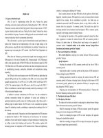
Table 1. Level of Per Capita Income (1990 Geary-Khamis dollars)

United States

Japan

South Korea

India

China

1955

10,970

2,695

1,197

665

818

1965

14,017

5,771

1.578

785

945

1975

16,060

10,973

3,475

900

1,250

Source: Maddison Angus, Monitoring the World Economy, 1820-1992. Washington, DC:
Organization for Economic Cooperation and Development, 1995, pp. 196-205.
The main purpose of the present paper is to develop an endogenous growth model that
combines structural change with repeated product improvements to discuss the issues of optimal
industrial structure, the (most) appropriate technology, and economic growth in an LDC in a

3

Hsieh and Klenow (2007) argues that both China and India would get big TFP (Total Factor Productivity) gains
from rationalizing allocation of capital and labor in both countries (TFP would double), while China appears to
have benefited from recent reform efforts, but India shows little gain.
3

dynamic general-equilibrium framework. Our paper pertains to work on structural change, i.e., the
systematic change in the relative importance of various sectors (e.g., Kuznets, 1957, 1973;
Chenery, 1960; Baumol, 1967; Laitner, 2000; Kongsamut, et al. 2001; and Ngai and Pissarides,
2007). In Kongsamut, et al. (2001), the production function of the different sectors, i.e.,
agriculture, services, and manufacturing, are proportional, while in Ngai and Pissarides (2007),
who focuses on exogenous total factor productivity differences across different sectors, all sectors
have identical Cobb-Douglas production functions. More closely related to our paper are
Acemoglu and Guerrieri (2006, 2008), Zhang (2006), as well as Zuleta and Young (2007).
Acemoglu and Guerrieri (2006) first illustrate, when the elasticity of substitution of different
products with different capital intensities in the aggregate production function of the final good is
not equal to unity, the inevitable outcome of directed technical change is non-balanced growth
between different sectors. Zuleta and Young (2007) developed a two-sector model of non-balanced
economic growth with induced innovation, in which one sector (“goods” production) has
technology differentiated by the elasticity of output with respect to capital and becomes
increasingly capital-intensive over time. 4 Zuleta and Young (2007) further assume that although
every technology is available at any instant, the adoption of a technology (i.e., innovation) is
costly and the cost of innovation is increasing in its capital, thus creating a tradeoff between
investment in capital and capital-intensity. In Zuleta and Young (2007), however, both the
investment in capital deepening, and the investment to adopt a more capital intensive production
function are the results of optimal decisions by an identical firm at any instant, and there is no
creative destruction, i.e., more advanced products render previous ones obsolete (Schumpeter,
1942, Segerstrom, et al. 1990, Grossman and Helpman, 1991a, and Aghion and Howitt, 1992). 5
There are two sectors in the present model, the traditional sector, and the modern sector.
Technological change in the traditional sector takes the form of horizontal innovation based on
expanding variety (Romer, 1990), while technological progress in the modern sector is
accompanied by incessantly creating advanced capital-intensive industry to replace backward
labor-intensive industry, which is the distinctive characteristic of the present model. Our paper is
the first attempt, to our knowledge, to address structural change with creative destruction, and to
simultaneously address the fact that some products in the modern economy – such as the personal
computer (PC) – become not only increasingly capita-intensive, but also progressively productive

over time.
The results of our model show that the optimal industrial structure in LDCs should not be the
same as that in DCs, the (most) appropriate technology adopted in the modern sector in LDCs
ought to be inside the technology frontier of the DCs, and the firm in the LDCs that enters
capital-intensive, advanced industry in the DCs would be nonviable owing to the relative scarcity
of capital in the LDCs’ factor endowments. Appropriate technology was first introduced by
Atkinson and Stiglitz (1969), and has been revived recently by Diwan and Rodrik (1991) as well
as Basu and Weil (1998). Basu and Weil (1998) is the first paper that provides the formal model to
discuss appropriate technology in the economic growth framework. The authors argue that
technology is specific to particular combinations of inputs, i.e., the capital-labor ratio in their
paper. Nevertheless, technological progress in Basu and Weil (1998) is the by-product of
4

Seater (2005) developed a one sector exogenous growth model with the similar technical change as in Zuleta and
Young (2007).
5
There is no change of capital-intensity in Segerstrom, et al. (1990), Grossman and Helpman (1991a), or Aghion
and Howitt (1992).
4


“localized learning by doing”, as introduced by Atkinson and Stiglitz (1969). In the present paper,
technological progress in the modern sector accompanied by increased capital intensity in the
generation of products requires an intentional investment of resources by profit-seeking firms or
entrepreneurs, which is emphasized in Grossman and Helpman (1994). Based on the endogenous
growth model with expanding variety, Acemoglu and Zilibotti (2001) argue that many
technologies used by LDCs are developed in the OECD economies and are designed to make
optimal use of the skills of the work force in the richer countries. Thus, the necessary outcome is
low productivity in the LDCs owing to the scarcity of skills in these countries. 6
The rest of the paper is organized as follows. Section 2 constructs a specific model of

endogenous economic growth that combines industrial structural upgrading with creative
destruction. In section 3, we investigate the issues of endogeneity of industrial structure and
appropriate technology as well as the firm’s viability in the LDC based on the dynamic trajectory
of the present economy. Section 4 contains some brief concluding remarks. Finally, some details
of the model that do not appear in the text are provided in the appendix.

2. The Basic Model
We consider a theoretical world consisting of a DC and an LDC that share the identical
demographics but have distinct factor endowment structures, 7 i.e., the relative abundance of
capital in the DC at time t0 , denoted by K (t0 ) , and the relative scarcity of capital in the LDC at
time t0 , denoted by K (t0 ) . To simplify the analysis, we assume there is no international trade
and no capital mobility in the present theoretical world.

2.1 Consumer Behavior
In both the DC and the LDC, there are L(t ) workers at time t , supplying their labor
without any disutility. 8 The population has a constant exponential growth rate g . We also assume
that all households share identical constant relative risk aversion (CRRA) preferences over total
household consumption index C (t , j ) , and all population growth takes place in existing
households, which implies that the economy admits a representative agent with CRRA
preferences:

U  





where

C (t , j )1  1

exp[  (t   )]dt
1

(1)

 is a subjective discount rate,   0 is the coefficient of relative risk aversion, and

6

There is never a problem of countries using technologies that do not match their level of development or
endowment structure in Basu and Weil (1998), while an LDC in Acemoglu and Zilibotti (2001) never has an
opportunity to choose his appropriate technology.
7
In the present paper, the upper bar is used as a superscript to indicate the variables in the DC, while the lower bar
is an index of the LDC.
8
We suppress time and country indexes when this causes no confusion.
5


C (t , j ) represents an index of consumption (sub-utility function) of j th generation goods at
time t . To reflect the household’s tastes for diversity in consumption, we adopt for C (t , j ) a
specification that imposes constant elasticity of substitution (CES) between consumption of
traditional goods, denoted by C1 , and consumption of modern goods of j th generation, denoted
by C2 (t , j ) . Specifically, we have
1


C (t , j )   C1  (1   )  C2 ( j )   , 0    1




where

(2)

  (0,1) is the share parameter of the two goods above, and   (0,1) determines the

elasticity of substitution between consumption goods in the traditional sector and in the modern
sector. It is convenient for us to choose traditional goods as numeraire and denote the price of
modern goods of j th generation to be p j .
The representative consumer maximizes (1) subject to an inter-temporal budget constraint.
The consumption optimization problem can be solved in two stages. First, the representative
consumer takes price p j as given and chooses C1 and C2 ( j ) to maximize static utility in (2)
for a given level of expenditure at time t , denoted by E (t ) .
1


max  C1  (1   )  C2 ( j )  

C1 ,C2 ( j ) 

subject to static budget constraint:

C1  p j C2 ( j )  E

(3)

The first-order conditions of the above maximization problem yield the following demand
functions for C1 and C2 ( j ) :

C1 

E
 (1   ) 
1 pj 

  p j 

1
 1

(4)

and

C2 ( j ) 

E
 (1   ) 


  p j 

(5)

1

 1

 pj

Substituting (4) and (5) into (2) yields

C ( j )  E  p j 

 

where  p j

amounts to
6








1


 1



(1

)

1  p


 
j 


  pj  



 

Substituting C ( j )  E p j



1


1

 
1


 (1   ) 

 (1   ) 
 p j  


 p 
j 

 


into (1), the representative agent’s utility function becomes

 E (t )  p j  


1

1

U  





1

exp[  (t   )]dt

(6)

The second-stage consumption optimization problem involves choosing the time pattern of
expenditures E to maximize (6) subject to the representative consumer’s inter-temporal budget

constraint:





t

exp[ R (t )  R ( x)]E ( x)dx  B (t )

(7)

where R (t ) is the cumulative nominal interest factor from time 0 to time t , i.e.,
t

R (t )   exp[r ( x)]dx with R (0)  1 , and B (t ) is the representative agent’s present value of
0

the stream of factor incomes plus the value of initial asset holding at time t .
The inter-temporal optimization problem of the above representative agent implies the
following Euler equation

E r (t )  


E

(8)

and the transversality condition

lim exp(  t ) (t ) B(t )  0
t 

where r (t ) is the nominal interest rate at time t .
Before leaving the consumption side of the economy, it will be useful for our later analysis to
consider the relationship of the representative consumer’s spending allocated to traditional goods
with respect to modern goods. Differentiating (3) with respect to time t yields

C1 C1 p j C2 ( j ) C 2 ( j ) p j C2 ( j ) p j E



C1 E
E
C2 ( j )
E
pj E
Denote the share of the representative consumer’s spending allocated to traditional goods by

s1 

p j C2 ( j )
C1
, and it is obvious that we have 1  s1 
, which is the share of the
E
E

representative consumer’s spending allocated to modern goods. Then we have

s1

p j E
C1
C ( j )
 (1  s1 ) 2
 (1  s1 )

C1
C2 ( j )
pj E

(9)

7


2.2 Producer Behavior and Static Equilibrium
Turning to the production side, there are only two primary factors of production, capital K
and labor L , and two sectors in both the DC and the LDC. One is the traditional sector and the
other is the modern sector. We assume the product in the traditional sector, denoted by Y1 , can be
used as consumption goods only, while the product in the modern sector, denoted by Y2 ( j )
which is the product of j th generation, can be consumed by households, installed by firms as
capital, or invested by entrepreneurs as R&D expenditures.
2.2.1 Production in the Traditional Sector
We assume that the production of the homogenous goods Y1 in the competitive traditional
sector only requires an index of intermediates D , and the production function of traditional
goods is

Y1  D
which is a standard assumption in the economic growth literature.
Following Grossman and Helpman (1991b), the index of intermediates D is represented by
N
D    z (i ) di 
 0


1

,

0  1

(10)

where z (i ) denotes the input of intermediate good i ; N is the number (measure) of available
intermediate goods, i.e., the technology in the traditional sector; and  is the elasticity of
substitution between different intermediate inputs. At every moment in time, the existing
producers of intermediate goods engage in oligopolistic price competition, and intermediate good

z (i ) is produced with the following Cobb-Douglas production function:
z (i )  l (i )  k (i )1  , 0    1

(11)

where l (i ) and k (i ) are labor and capital employed in the production of the existing
intermediate good z (i ) .
Facing the given price of the existing intermediate good z (i ) , which is denoted by q (i ) ,
and the price for the product of the traditional sector, which is normalized to be 1, the inverse

demand function for the existing intermediate good z (i ) by the competitive firm in the
traditional sector is given by:

q (i )  (Y1 )1 z (i ) 1

(12)

8


And the profit maximization problem of the existing intermediate firm i can be
equivalently written as

Max (Y1 )1 .l (i ) k (i ) (1  )  w.l (i )  r.k (i )

(13)

l ( i ), k ( i )

The first-order conditions in (13) are

 (Y1 )1 .l (i ) 1 k (i ) (1  )  w

(14)

 (1   )(Y1 )1 .l (i) k (i ) (1  ) 1  r

(15)

Combining (14) with (15) yields the existing intermediate firm i ’s factor demand functions

1

l (i )  (1   ) (1  )  (1  )  w (1  ) r  (  ) (Y1 )(1 )  1
k (i ) 

1
w(1   )
(1   ) (1  )  (1  )  w (1  ) r  (  ) (Y1 )(1 )  1
r

(16)

(17)

Substituting existing intermediate firm i ’s factor demand functions in (16) and (17) into (12),
then q (i ) , i.e., the price of the existing intermediate good z (i ) , satisfies

q(i )   1 (1   )  (1  )    w r1 

(18)

Thus, in a symmetric equilibrium, all the existing intermediate firms in the traditional sector
would charge the same price and share identical factor demand functions, which implies

l (i ) 

L1
K
and k (i )  1
N

N

(19)

where L1 and K1 are the total amount of labor and capital used in the traditional sector,
respectively.
1

L1  N  (1   ) (1  )  (1  )  w (1  ) r  (  )  1 Y1
K1  N

1
w(1   )
 (1   ) (1  )  (1  )  w (1  ) r  (  )  1 Y1
r

(20)

(21)

Now the production function of the existing intermediate good z (i ) in (11) becomes

z (i ) 

1

1 
 L1   K1 
N

(22)

and the production function of the traditional sector in (10) could be rewritten as

Y1  N

1



 L1   K1 


(1  )

(23)

Combining (19) and (23) with (14) and (15) implies the wage rate and interest rate satisfy

w   N

1



r   (1   ) N

 K1
1



L1 

 K1

1 

L1 

(24)


(25)

9


Substituting (24) and (25) into (13), the profit function of the existing intermediate firm i in
the traditional sector can be obtained by

 1 (i )  (1   ) N

1 2



 L1   K1 


1 

(26)

As in Judd (1985) and Romer (1990), we also assume that production of a new intermediate
good requires R&D expenditures X 1 in terms of the modern goods devoted to the invention of a
new blueprint. Moreover, we also assume that process innovation outlays are made by private,
profit-making entrepreneurs, who receive indefinite patent protection and will appropriate some of
the benefits from a new process innovation in the form of oligopoly profits. The oligopolistic
entrepreneur of intermediate firm i in the traditional sector’s present value of future operating
profits from producing z (i ) discounted to time t is given by


V1 (i, t )   exp[ R(t )  R( x)] 1 (i, x) dx
t

where

 1 (i, x) is the flow profits of firm i from producing intermediate good z (i) in the

traditional sector, which is expressed by (26) at time x .
Differentiating V1 (i, t ) with respect to time t yields

V1 (i, t )
 (i, t )
r 1
V1 (i, t )
V1 (i, t )

(27)

With the spillover effect from the current stock of knowledge in the traditional sector to
future process innovations emphasized in Romer (1990) in mind, we assume that if X 1 units of
modern goods engage in research in the traditional sector, they generate a flow of new products

N given by
N  b1 N 1 X 1
where b1 is a strictly positive constant measuring the technical difficulty of creating new
blueprints in the traditional sector, and

1  (1, ) measures the degree of spillovers in

technology creation.
Then, with free entry by the intermediate firm i , if there are positive but finite resources
devoted to R&D in the traditional sector at time t , we must have the zero-profit condition for
firm i as

V1 (i, t )  p j

N 1
b1

(28)

2.2.2 Production in the Modern Sector

10


Producing the product in the modern sector also requires variable inputs capital K and

labor L , but not intermediates. The production function of the product of j th generation in the
modern sector is given by
 1
Y2 ( j )  F2 [ A2 ( j ), K , L]  A2 ( j ) K 2 j L2 j , 1     j  

where  is an exogenously given parameter that satisfies

  1 , K 2 , L2 and  j is capital

and labor used, as well as the capital intensity in the modern sector for the product of j th
generation, respectively, and A2 ( j ) is the productivity of the j  1, 2,... th generation product.
The parameters in the present paper that satisfy 1     j   imply that the modern sector is
more capital-intensive than the traditional sector at any moment.
Following the literature on horizontal innovation or creative destruction (e.g., Segerstrom, et
al., 1990; Grossman and Helpman, 1991a; as well as Aghion and Howitt, 1992), we assume the
productivity of the j  1, 2,... th generation in the modern sector, denoted by A2 ( j ) , is exactly

 times that of the generation before it. That is, we have
A2 ( j )   A2 ( j  1)
where

 is an exogenously given constant that satisfies   1 . We choose units so that the

productivity of the lowest generation with j  0 , i.e., the one available at time t  0 (the
starting point of the analysis), is equal to unity; that is we assume A2 (0)  1 . 9
In contrast with the literature on horizontal innovation or creative destruction mentioned
above – which focus on productivity (or product quality) rising only – the present paper embodies
product innovation in technological progress that is incessantly capital intensive and progressively
productive over time. We assume that the relationship between capital intensity
generation

 j of the

j  1, 2,... with that of generation j  1 satisfies the following condition for

simplicity

 j   j 1  b2 (   j 1 )
where b2  0 and

3

(29)

3  0 . 10

Now the production function in the modern sector could be rewritten as
As the starting point of the analysis, we assume that the modern sector begins at time t  0 with one firm
which has access to a universally known backstop technology in the perfectly competitive output market and factor
market until the first generation product is invented.

9

10

Equation (29) implies in infinite horizon we have

lim  j (t )  lim  j   .
t 

j 

11




1 j

Y2 ( j )  F2 [ A2 ( j ), K , L]   j K 2 j L2

(30)

Of course, more advanced products, i.e., products with higher productivity and rising capital
intensity, could not be produced until they have been invented. We follow the approaches taken in
Aghion and Howitt (1992) as well as in chapter 4 of Grossman and Helpman (1991b), and assume
that research in the modern sector produces a random sequence of product innovations. Any firm
in the modern sector that carries out R&D at intensity  for a time interval of length dt will
succeed in its attempt to develop the product of generation j  1, 2,... based on the existing
generation before it with probability

 dt which follows a Poisson distribution. R&D
j 2

expenditures per unit of time in this activity are X 2  ( )
the entrepreneur attempts to develop the product, where

 in terms of modern goods when

2  1 (1   )  1 reflects the fact that

the more advanced the technology in modern sector, the more R&D expenditures are needed for
further product innovation in this sector. Furthermore, we assume the parameters of the present
model satisfy

 (1  1 )   2 (1   )(1   ) to guarantee balanced growth between the

traditional sector and the modern sector on the infinite horizon. 11
Once the product of generation j  1, 2,... has been invented in the research lab, the
successful innovator obtains a patent that is assumed to last forever on condition that no new
generation has been invented; otherwise, the present generation product in the modern sector will
be replaced by the next generation/vintage. And the producers with the requisite know-how and
patent rights can manufacture the product of j th generation in the modern sector according to the
production function in (30). We assume that all firms in the modern sector engage in price
competition in the output market and are price-takers in the factor market, and we also assume that
only one leader-firm, e.g., firm j , in the modern sector has access to the state-of-the-art
technology. Another firm, a follower-firm, i.e., firm j  1 , masters the technology that is one step
behind it.
For the moment, we assume innovations are always drastic, which means the successful
innovator is unconstrained by potential competition from the previous patent. 12
From (4) and (5), the inverse demand function faced by a monopolistic firm j in the
modern sector charging price p j can be solved as follows:

(1   )  C2 ( j ) 
pj 
 C1 1

 1

Let us denote the fraction of modern goods of the j th generation consumed by households

11

When

 (1  1 )   2 (1   )(1   ) , non-balanced growth between the traditional sector and the

modern sector implies that either the traditional sector or the modern sector will be trivial compared to the other
sector in infinite horizon.
12
Please see Lin and Zhang (2007b) for the details of the case of nondrastic innovations.
12


by

j 

C2 ( j ) 13
, then we have
Y2 ( j )
(1   )   jY2 ( j ) 

 1

pj 

(31)

 C1 1

Facing the given inverse demand function in (31), given factor prices w j and rj , the firm

j in the modern sector will choose K 2 and L2 to maximize profit, given by:
(1   )   j 

 1

 2 ( j) 

 K
j

 C1 1



 j 1 j 

L2

2

 rj K 2  w j L2

(32)

The first-order conditions in (32) are

(1   )   j 

 1

 j

 C1

 1

(1   )   j 

 1

 j

 C1

 1

 j 1  (1 j )

 j K 2

L2

 j

 rj

 (1 j ) 1

 (1   j ) K 2 L2

(33)

 wj

(34)

Combining (33) with (34) implies that the factor demand functions of firm j in the modern
sector should satisfy
1

 (1   )    1  j
1
j

(1 j )
 (1 j )
  j 
 j
L2  
 (1   j )
( j ) ( w j )
( rj ) 
 C1 1


K2 

 j wj
L2
(1   j )rj

(35)

(36)

Substituting (35) and (36) into (32), we can solve the profit function of firm j in the
modern sector as follows

(1   )   j 

 1

 2 ( j )  (1   )

 j

 C1 1

K



 j 1 j 
2

L2

(37)

And the price of the product of the j th generation in the modern sector is determined by

p j    j 1  j 

 j

(1   j )

 (1 j )

(w j )

(1 j )

j

( rj )

(38)

At time t , the value to an outside research firm j that aims to develop a product whose
productivity is

 times as great as the state of the art and carries out R&D at intensity  when

this firm is successful in the j th product innovation, which is denoted by V2 ( j , t ) , is the
expected present value of the flow of monopoly profits
13

It is obvious that

1  j

 2 ( j, x) discounted to time t , where

denotes the savings rate in the present model.
13


the duration of

 2 ( j, x) follows the exponential distribution with parameter  x :


V2 ( j , t )   exp[ R(t )  R ( x)] 2 ( j , x) ( j , x)dx
t

where

 ( j , x)

equals the probability that there will be exactly j innovations from the

starting point to time x , thus, we have

( x) j e  x
 ( j, x)  j !
Newcomer firm j in the modern sector would choose research intensity  for a time

interval of length dt to maximize

max V2 ( j , t ) dt  p j (t )( j )2  dt


(39)

The maximization problem in (39) implies

p j (t )( j )2  V2 ( j , t ),   0 and  p j (t )( j )2  V2 ( j , t )    0
Thus, as long as the R&D operates at a positive but finite scale, we must have

  0 , and

p j (t )( j )2  V2 ( j , t ) . And the variation of the value to an outside research firm j discounted
to time t , denoted by V2 ( j , t ) , can be expressed as

V2 ( j , t )
 ( j, t )
 r   2
V2 ( j , t )
V2 ( j , t )

(40)

2.3 Market Clearing Conditions
We close the model by describing market clearing conditions. The output market clearing
condition in the traditional sector implies

C1  Y1

If we neglect capital depreciation in our model for simplicity, then the output market clearing
condition in the modern sector is:

C2 ( j )  K  X 1  X 2  Y2 ( j )
According to the analysis above, the factor market clearing conditions can be expressed as:

L1  L2  L
K1  K 2  K
where L1 ( K1 ) and L2 ( K 2 ) denotes the levels of labor (capital) used in the traditional and
modern sectors, respectively. It is convenient for the analysis below to denote the fraction of labor

14


and capital used in the traditional sector by

L 

L1
K1
and  K 
. From (20),
L1  L2
K1  K 2

(21), (35), and (36), we find

L 

1

 1
1
 (1 j )
  

(1 j )
j
( j ) j ( w j )
( rj ) j 
  (1   )   j    (1   j )

1 

1
1

(41)

1

N (1   ) (1  )  (1  )  w (1  ) r  (  )  1
and

K 

1
1

1
 1

1
(1 j )

 (1 j )
  
j
( j ) j ( w j )
( rj ) j 
  (1   )   j    (1   j )

1 
1

r

(1
)
w(1   )
j
j
 (1  ) (1  )
 (1  )  (  ) 1

N (1   )
r

w
r
 j wj

Since the traditional sector and the modern sector share the identical factor prices in
equilibrium, we have

K 

where

j 

L
 L   j (1   L )

(42)

 j
. Thus,  L could characterize the industrial structure in the present
(1   j )(1   )

model.

2.4 Dynamic Equilibrium with an Infinite Horizon
The dynamic equilibrium in this economy is given by paths for prices of factors,
N

intermediates and modern goods w , r , [q (i )]i 1 , p , allocations of factors L1 , L2 , K1 ,

K 2 , as well as R&D expenditures X 1 , X 2 such that producers maximize profits, and the
representative consumer chooses consumption and savings C1 , C2 and E to maximize his
utility under the market clearing conditions. It is convenient for us to study equilibrium with an
infinite horizon first, and then characterize the dynamic trajectory of the present economy. As

regards equilibrium with an infinite horizon, we have the following prosposition (see the
Appendix for the proof).
Proposition 1: There exists a constant growth equilibrium (CGE) in the present economy
*

with an infinite horizon, which means consumer expenditures E grow at a constant rate g E

15


with an infinite horizon, i.e., lim
t 

E
 g E* , and the interest rate in CGE is also a constant, i.e.,
E

lim r  r *   g E*   . Furthermore,  (1  1 )   2 (1   )(1   ) implies that the CGE is
t 

also a unique balanced growth equilibrium (BGE), such that the modern sector and the traditional
sector grow at the same constant rate with an infinite horizon, where

Y1
 (1  1 )
Y
 (1   )
 gY*1 
g , lim 2  gY*2  2
g , and g E*  gY*1  gY*2 .


t  Y
t

 (1  1 )  (1   )
Y2
2 (1   )  1
1

lim

3. Industrial Structure, Appropriate Technology,
and Firm Viability in LDCs
In this section, we will explore the issues of endogenous industrial structure, appropriate
technology and viability of a firm in the LDCs based on the dynamic trajectory of the above basic
model.

3.1 Structural Change and Technological Progress in the Dynamic Trajectory
Now we begin with the dynamic trajectories of the economy described in the present paper.
The dynamic trajectories of this economy can be characterized by an autonomous system of

E

nonlinear differential equations which contains three control variables, e 

1

LN

, X 1 , and


(1 1)  (1 )

X 2 as well as seven state variables,  ,  L , p ,  , k 

K
1

LN



,

n

N



L

,

t

and  



0

( 2 )  ( x ) dx

L

(1 )(   1)

N

.



First and foremost, we need to solve the equilibrium interest rate r in the dynamic
trajectories. From (25), we know that the equilibrium interest rate in the dynamic trajectories is
determined by:

   (1   ) L 
r   (1   ) 

k

where






1.
(1   )(1   )

Second, we need to calculate the dynamics of capital intensity in the modern sector. We could
invoke the property of a Poisson distribution to argue that the expected time of a firm in the
modern sector that carries out R&D at intensity

 (t ) to develop the product of generation
16


j  1, 2,... based on the existing generation before it is dt  1  (t ) (Feller, 1968). Therefore,
from (29), the dynamics of capital intensity in the modern sector, denoted by  , is given by

(t )  lim

 (t  dt )   (t )

dt 0

 b2 [   (t )]3  (t )

dt

(43)

Third, we should discover the evolution of the optimal R&D intensity in the dynamic paths.
t


Differentiating p 0

2  ( x ) dx

 V2 (t ) with respect to time t implies
V (t )
p
  2 ln  (t )  2
p
V2 (t )

(44)

Combining (40) with (44), we obtain

p  2 (t )

p V2 (t )

( 2 ln   1)  r 

where

 2 (t )
V2 (t )

 (1   )

(1   )   1 (1   K ) (1   L )(1 )  (1  )( 1)

k
.
 (  1)
(1  )(  1)
p
 L 
 K 

Thus, the evolution of normalized accumulated R&D intensity, denoted by  , should satisfy



where

K 

p
(1   )   1 (1   K ) (1   L )(1 )  (1  )( 1)
r   (1   )
k
 ( 1)
(1  )(  1)
p
p
 L 
 K 

(45)

( 2 ln   1)

L
.
 L   (1   L )

Fourth, we need to characterize the evolution of technology in the traditional sector.
Differentiating the zero-profit condition for firm i in the traditional sector, which is expressed by
(28) with respect to time t , yields

V1 (i, t ) p
N
  1
V1 (i, t ) p
N

(46)

 (i, t )
p
N
 1  r  1
p
N
V1 (i, t )

(47)

Combining (27) with (46) yields

(1   )  L   K 

Substituting
 b1
V1 (i, t )
p

 1 (i, t )



1 

k

1 

n

 n



N


and
N (1  1)  (1   )

   g 
n

into (47) implies the dynamics of normalized technology in the traditional sector, denoted by

n
,
n

is determined by

17


 n




1 
(1   )  L   K  k 1 
p

 1
 r  b1
(1  1)  (1   )
p
p
n

   g 
n

Fifth, from (41), we obtain the fraction of labor used in the traditional sector
1

1

 1

L

1

 (1   )  1 1
1
1


(1

)


 




 (1  ) (1  )

 
(1   )



k


   (1   ) L 

1
1

( )

 
(1 )(1 )

 ( 1  )
1

 1  
  



(48)

 L as


(n)

( 2 )(1 )

  (  1)

1
1

(49)

Sixth, it is time for us to understand the law of price change in the present model. From (31),
the price of the product in the modern sector can be rewritten as


(1   )   (t ) K 2 L12
p
  1  1 
 N L1 K1







 1

(50)

Differentiating (50) with respect to time t , we obtain the law of the price of modern goods,

denoted by

p
, as
p

 
k
(1   )(  1)
 n

   ln       1 
  g  

k  (1  1)  (1   )  n
p

 (  1) 


p
 K




 (1   ) L   L  (1   ) K


1 K

1 L
L
K



(51)

 (1   K ) K 
where  ln 
 is infinitesimal and we neglect it in (51).
 (1   L ) L 

Seventh, the Euler equation of the representative agent requires that the optimal path for the
normalized consumption expenditure e must satisfy

 n

(1   )   g 
e r  
n


 g 
e
(1  1)  (1   )


(52)

Eighth, from (9), the dynamics of the fraction of modern goods consumed by households



could be determined by

18




 n

2(1   )    g 



r
n
    k   K   g  (1   )  L   (1  s ) p
 s1 


1

L 
p
 (1  1)  (1   )
 k K 





 n  
(1
)



 g

 




k
n
   K  g  (1   ) L 
 (1  s1 )    ln  

1 L 
k (1  1)  (1   ) 1   K



where s1


1 

 L   K 



e

(53)

(1   K ) K
k 1  and again we neglect b2 [   ]3  ln
, which is
(1   L ) L

infinitesimal, in (53).
Ninth, the market clearing condition in the modern sector implies the dynamics of normalized
capital, denoted by

k
, follows
k
1
k
 2  1

1
 (1   )(1   K ) (1   L ) (n)
k
k
  n
  n


2

 1     g 

 2  2
bk
 n 

 n

 g   1
(1  1)  (1   )
k

(54)

Finally, the other two control variables X 1 and X 2 can be computed as X 1 

1  1
NN
b1

t


and X 2   0

2  ( x ) dx

 with the initial value of technology in the traditional sector at the starting

point of the analysis, i.e., the exact value of N (t ) at time t  0 , denoted by N (0) , as well as

A2 (0)  1 assumed above.
Summarizing the results above, we can characterize the dynamics of the present economy as
well as industrial structural change and technological progress in the following proposition.
Proposition 2: The dynamic equilibrium of the present economy could be characterized by
an autonomous system of nonlinear differential equations which contains eight variables,

 , ,

n ,  L , p , e ,  , and k , given by eight equations (43), (45), (48), (49), (51), (52), (53), (54).
Furthermore, in both LDCs and DCs, the evolution of industrial structure
appropriate technology N (t0 ) , j (t0 ) ,

 L (t0 ) and

 (t0 ) at time t  t0 is endogenously determined by

the above autonomous system of nonlinear differential equations, as well as the capital stock

K (t0 ) at time t  t0 and initial conditions in labor and technology in the traditional sector and
19


the modern sector, i.e., L(0) , N (0) , and

 0 at the starting point of the analysis t  0 .

3.2 Catch-up and Firm Viability in LDCs
It is obvious from proposition 2 that we have

 L (t0 )   L (t0 ) ,  (t0 )   (t0 ) ,

j (t0 )  j (t0 ) , and n (t0 )  n (t0 ) when K (t0 ) K (t0 )  1 at time t  t0 . The ratio of capital
in the DC to that in the LDC, denoted by K K , could be interpreted broadly, as a metaphor for
the LDC’s current stage of development. The larger K K is, the more backward the economy in
this LDC, and K K will decrease and approach unity eventually as the LDC converges to the
DC. Moreover, the ratio of technology in the DC to that used in the LDC denotes the distance to
the technology frontier in the LDC, where N N denotes the distance to the technology frontier
of the traditional sector, and j j denotes the distance to the technology frontier of the modern
sector. When these terms are large, the LDC is far from the world technology frontier.
As pointed out in section 1, motivated by the dream of nation building, most of the LDC
governments pursued a catch-up type strategy to accelerate the development of the then advanced
capital-intensive industries after World War II. Thus, in reality, the actual industrial structure and
technology adopted in LDCs may deviate from that endogenously determined in proposition 2. If
we define the industrial structure and technology in an LDC endogenously determined in
proposition 2 as the optimal industrial structure and (most) appropriate technology in that country,
by summarizing the analysis above, we obtain the following result.
Corollary 1: Owing to the relative scarcity of capital in LDCs, endogenous industrial
structural change and technological progress on the dynamic trajectory imply that the (optimal)
industrial structure in LDCs should not be the same as that in DCs; the (most) appropriate
technology adopted in the modern sector in LDCs ought to be inside the technology frontier of the
DCs.
On the viability of the firm in the government’s priority industries when this government
pursued a catch-up type strategy to accelerate development of the then advanced capital-intensive
industries, we obtain the following proposition.
Proposition 3: When an LDC government pursues a catch-up type strategy, the firm in this
LDC that enters a capital-intensive, advanced industry of the modern sector in the DCs would be

nonviable owing to the relative scarcity of capital in the factor endowments of the LDCs.
Proof: We will prove proposition 3 based on an extreme assumption first, then extend it to
the general case. The extreme assumption is that we model the catch-up type strategy in the LDC
whose capital stock equals to K (t0 ) at time t  t0 by assuming that the actual industrial
structure and technology chosen by the government in the LDC coincides with those in the DC
whose capital stock equals K (t0 ) at time t  t0 for tractability, i.e., N (t0 )  N (t0 ) ,
20


j (t0 )  j (t0 ) ,  (t0 )   (t0 ) , and  L (t0 )   L (t0 ) at time t  t0 , when K (t0 )  K (t0 ) .
From the analysis in subsection 2.2, we know that, without external subsidies, as long as
R&D operates at a positive but finite scale, the present value of firm j in any country
discounted to time t0 , denoted by V2 ( j , t0 ) , must satisfy the free-entry condition, i.e.,

p j (t0 )( j )2  V2 ( j , t0 ) . Naturally, the present value of the firm in the DC, whose capital stock
equals K (t0 ) , which enters industry j discounted to time t0 , denoted by V2 ( j , t0 ) , meets
the above free-entry condition precisely, because there is positive and bounded R&D intensity in
the DC, which implies that we have

p j (t0 )( j )2  V2 ( j , t0 )

(55)

Equation (40) could be reformulated as

V2 ( j , t ) V2 ( j , t )
 ( j, t )

 2
(r   ) p j (r   ) p j

pj
Substituting

 2 ( j)
pj

(56)

 (1   )Y2 ( j ) into (56) yields

V2 ( j , t ) V2 ( j , t ) (1   )Y2 ( j , t )


pj
(r   ) p j
(r   )

where

p j
K

  (t )


1
(1   )   [(1   K ) K ] [(1   L ) L]   X 1  X 2  
pj 
1


 

1 


N
(

L
)
(

K
)


L
K

(57)
 1

and

satisfies

0.
Differentiating (57) with respect to K obtains

 

V2 ( j , t )  K V2 ( j , t ) V2 ( j , t ) r




(r   ) p j
(r   ) 2 p j K
 p j 
V2 ( j , t ) p j (1   ) Y2 ( j ) (1   )Y2 ( j ) r


(r   )( p j ) 2 K (r   ) K
(r   ) 2 K

K

It is obvious that V2 ( j , t )  0 ,


K

(58)

Y2 ( j )
r
0,
 0 , which imply that we have
K
K

V2 ( j , t ) 
 
V2 ( j , t ) is a higher-order infinitesimal term which could be

  0 , owing to
K
 p j 

neglected in (58). Therefore, given N (t0 )  N (t0 ) ,

j (t0 )  j (t0 ) ,  (t0 )   (t0 ) , and
21


 L (t0 )   L (t0 ) at time t  t0 , p j (t0 )( )  V2 ( j , t0 ) is a direct conclusion from (55)
j

2

when K (t0 )  K (t0 ) , which means that the firm in the modern sector of the LDC would be
nonviable if this LDC imitates the industrial structure and copies the most advanced technologies
used in the DC exactly.
Furthermore, as a matter of fact,

V2 ( j , t )
is a continuous function of all its arguments, thus,
pj

when there is a severe scarcity of capital in the LDC, i.e., K (t0 ) K (t0 ) is much greater than 1,
the conditions that N (t0 )  N (t0 )   N ,

when

 N  0 ,  j  0 , and 

j (t0 )  j (t0 )   j , and

 L (t0 )   L (t0 )  

are all small enough, could still suffice for

p j (t0 )( )2  V2 ( j , t0 ) , thereby we would obtain proposition 3.
j

Q.E.D.

Therefore, it is imperative for the government to introduce a series of regulations and
interventions to mobilize resources for setting up and supporting the continuous operation of the
non-viable firms. This type of economy might become very inefficient as the result of
misallocation of resources (Lin, 2007, Lin and Zhang, 2007a).

4. Concluding Remarks
In the present paper, we have developed an endogenous growth model that combines
structural change with repeated product improvements. The distinctive characteristic of our model
originates from the technology in the modern sector, which becomes not only increasingly
capital-intensive, but also progressively productive over time as the result of innovation by the
profit-seeking firms. Each technology in the modern sector is appropriate for one and only one
capital-labor ratio, i.e., the technologies in the modern sector are specific to particular factor
endowment structures. Therefore, we could draw the conclusion that an LDC’s optimal industrial
structure and the (most) appropriate technology are endogenously determined by that economy’s
endowment structure, and the optimal industrial structure in LDCs should not be the same as that

in DCs. That is, the (most) appropriate technology adopted in the modern sector in the LDCs
ought to be inside the technology frontier of the DCs, and a firm in an LDC that enters
capital-intensive, advanced industry in a DC would be nonviable owing to the relative scarcity of
capital in the factor endowments of LDCs. We hope the framework developed in the present paper
provides a new line of thought for analyzing the root cause of the differences in economic
performance in LDCs. Our argument is that whether the industrial structure and technology
adopted in LDCs match the factor endowment structure is the fundamental reason for the diversity
in economic performance among LDCs.

22


References
Acemoglu, Daron and Veronica Guerrieri. “Capital Deepening and Non-Balanced Economic
Growth”, (August, 2006). NBER Working Paper No. W12475, Available at SSRN:
/>Acemoglu, Daron and Veronica Guerrieri. “Capital Deepening and Non-Balanced Economic
Growth”, Journal of Political Economy，Vol.116, No. 3. (June 2008), pp. 467-498.
Acemoglu, Daron, and Fabrizio Zilibotti, “Productivity Differences”, Quarterly Journal of
Economics, Vol. 116, No. 2. (May, 2001), pp. 563-606.
Aghion, Philippe and Peter Howitt. “A Model of Growth through Creative Destruction”,
Econometrica, Vol. 60, No. 2. (Mar., 1992), pp. 323-351.
Arrow, Kenneth J. “The Economic Implications of Learning by Doing”, Review of Economic
Studies, Vol. 29, No. 3. (Jun., 1962), pp. 155-173.
Atkinson, Anthony B and Joseph E. Stiglitz. “A New View of Technological Change”, Economic
Journal, Vol. 79, No. 315. (Sep., 1969), pp. 573-578.
Barro, Robert J. and Xavier Sala-i-Martin, Economic Growth, 2nd Edition. Cambridge: MIT Press.
(2003).
Basu, Susanto. and David N. Weil. “Appropriate Technology and Growth”, Quarterly Journal of
Economics, Vol. 113, No. 4. (Nov., 1998), pp. 1025-1054.
Baumol, William J. “Macroeconomics of Unbalanced Growth: The Anatomy of Urban Crisis”,

American Economic Review, Vol. 57, No. 3. (Jun., 1967), pp. 415-426.
Caselli, Francesco and Jaume Ventura. “A Representative Consumer Theory of Distribution”,
American Economic Review, Vol. 90, No. 4. (Sep., 2000), pp. 909-926.
Cass, David. “Optimum Growth in an Aggregative Model of Capital Accumulation”, Review of
Economic Studies, Vol. 32, No. 3. (Jul., 1965), pp. 233-240.
Chenery, Hollis B. “Patterns of Industrial Growth”, American Economic Review, Vol. 50, No. 4.
(Sep., 1960), pp. 624-654.
Diwan, Ishac and Dani Rodrik. “Patents, Appropriate Technology, and North-South Trade”,
Journal of International Economics, Vol. 30, Issue, 1-2, (February, 1991), pp. 27-47.
Ericson, Richard E. “The Classical Soviet-Type Economy: Nature of the System and Implications
for Reform”, Journal of Economic Perspectives, Vol. 5, No. 4. (Autumn., 1991), pp. 11-27.
Feller, William. “An introduction to probability theory and its applications”, 3rd Edition, New York:
John Wiley, 1968.
Grossman, Gene M. and Elhanan Helpman. “Quality Ladders in the Theory of Growth”, Review
of Economic Studies, Vol. 58, No. 1. (Jan., 1991a), pp. 43-61.
Grossman, Gene M. and Elhanan Helpman. Innovation and Growth in the Global Economy,
Cambridge: MIT Press. (1991b).
Grossman, Gene M. and Elhanan Helpman. “Endogenous Innovation in the Theory of Growth”,
Journal of Economic Perspectives, Vol. 8, No. 1. (Winter, 1994), pp. 23-44.
Hsieh, Chang Tai and Peter Klenow, “Misallocation and Manufacturing TFP in China and India”,
(May, 2007). Available at: />Jones, Larry E. and Rodolfo E. Manuelli. “A Convex Model of Equilibrium Growth: Theory and
Policy Implications”, Journal of Political Economy, Vol. 98, No. 5, Part 1. (Oct., 1990), pp.
1008-1038.
Judd, Kenneth L. “On the Performance of Patents”, Econometrica, Vol. 53, No. 3. (May, 1985), pp.

23