Business Cycles in the Eastern Caribbean Economies The Role of Fiscal Policy and Interest Rates
Bạn đang xem bản rút gọn của tài liệu. Xem và tải ngay bản đầy đủ của tài liệu tại đây (1.13 MB, 32 trang )
Public Disclosure Authorized
Public Disclosure Authorized
Policy Research Working Paper
7545
Business Cycles in the Eastern Caribbean Economies
The Role of Fiscal Policy and Interest Rates
Francisco Carneiro
Viktoria Hnatkovska
Public Disclosure Authorized
Public Disclosure Authorized
WPS7545
Macroeconomics and Fiscal Management Global Practice Group
January 2016
Policy Research Working Paper 7545
Abstract
This paper analyzes the business cycle characteristics of
the economies of the Organization of Eastern Caribbean
States using a model of a small open economy subject to
interest rate and fiscal expenditure shocks and financial
frictions. The paper shows that macroeconomic aggregates in this region are quite volatile, with consumption
exhibiting higher volatility than gross domestic product.
The analysis also finds that in these economies real interest rates are highly volatile and strongly countercyclical
with gross domestic product and other macroeconomic
aggregates. Similarly, fiscal expenditures show significant
volatility, but are pro-cyclical with gross domestic product. The results suggest two major directions for designing
policies to help reduce the volatility experienced by the
Organization of Eastern Caribbean States economies. First,
Organization of Eastern Caribbean States countries should
seek a greater openness to international financial markets,
which could help them smooth out the effects of fundamental shocks, such as shocks to technology and terms of
trade, and shocks associated with natural hazards. However, this removal of international financial barriers needs
to be accompanied by improvements in domestic financial
conditions, as this would reduce the vulnerability of these
economies to country risk premium shocks. Second, the
Organization of Eastern Caribbean States region should
try harder to move toward a countercyclical fiscal policy
stance, as this could help to stabilize the domestic risk
premium and cushion the negative effects of interest rate
shocks on economic activity, hence reducing volatility.
This paper is a product of the Macroeconomics and Fiscal Management Global Practice Group. It is part of a larger effort
by the World Bank to provide open access to its research and make a contribution to development policy discussions
around the world. Policy Research Working Papers are also posted on the Web at . The authors
may be contacted at
The Policy Research Working Paper Series disseminates the findings of work in progress to encourage the exchange of ideas about development
issues. An objective of the series is to get the findings out quickly, even if the presentations are less than fully polished. The papers carry the
names of the authors and should be cited accordingly. The findings, interpretations, and conclusions expressed in this paper are entirely those
of the authors. They do not necessarily represent the views of the International Bank for Reconstruction and Development/World Bank and
its affiliated organizations, or those of the Executive Directors of the World Bank or the governments they represent.
Produced by the Research Support Team
Business Cycles in the Eastern Caribbean Economies: The Role of Fiscal
Policy and Interest Rates
Francisco Carneiro*
and
Viktoria Hnatkovska†
Keywords: Eastern Caribbean States, volatility, business cycles
JEL Classification: E30, O11, O54
*
Lead Economist and Program Leader, Caribbean countries, the World Bank, 1818 H Street - I 8-804 - Washington,
DC 20433 USA;
†
University of British Columbia, 1017-1873 East Mall, Vancouver, BC V6T1Z1, Canada,
, corresponding author.
1. Introduction
The Caribbean region is home to some of the smallest states in the world. Although similar
in their smallness, there are marked differences among them. Caribbean nations differ in size,
income levels, and economic structure. 1 In terms of economic structure, the region hosts a few
commodity-exporters (such as the Dominican Republic, Guyana, Belize, Suriname, and Trinidad
and Tobago) while others are service-oriented economies (such as Barbados, Grenada, Bahamas,
St. Lucia and others). Similarities include proximity to major markets in North and South America,
and for most countries, a transition from agriculture or mining to a service-driven economy,
anchored in particular on tourism and financial services. Common challenges include exposure to
frequent natural disasters; vulnerability to external shocks; high debt; and lack of economies of
scale.
The commodity-exporting group has done very well until recently when commodity prices
started to fall, with most of the countries showing high growth, solid fiscal stances, and sustainable
debt levels. Now, with the end of the commodity super-cycle, these countries are facing fiscal
pressures and their debts are increasing. The tourism-based economies, on the other hand, were
the ones suffering the most with low growth rates since the global financial crisis that led to low
tourism, low remittances, high non-performing loans in banks, and considerable fiscal strain. They
are now the ones who stand to benefit the most from the current state of affairs as oil prices remain
low and the main sources of tourism-related revenues and remittances, namely the US, Canada,
and Europe, start to grow faster.
Because the tourism-dependent countries are the smallest open economies in the region,
they tend to suffer the most with volatility associated with terms of trade shocks. The members of
the Organization of Eastern Caribbean States (OECS)2 are especially vulnerable. Their growth
performance has been uneven over the last three decades or so due to reasons that range from the
need to reinvent themselves after the end of preferential trade agreements with Europe in the 1980s
to the occurrence of natural hazards. After growing faster than the rest of the world in the 1980s
at an annual average of 6 percent, the OECS countries have experienced a significant growth
slowdown since the 1990s with annual growth rates of 2 percent or less on average. More recently,
the region was severely hit by the effects of the global financial crisis of 2008-09 because of their
close ties with the economies of the U.S., Canada, and Europe which are their main source of
tourist arrivals.
Understanding the sources and consequences of macroeconomic volatility comprises one
of the key challenges facing policy makers in developing countries, and especially so in small
island states. The main objective of this paper, therefore, is to provide an in depth exploration of
the sources of macroeconomic volatility in the Eastern Caribbean economies, contrast them with
other developing economies, and evaluate their effects on the macroeconomic performance of
1 From
the small island states of the Organization of the Eastern Caribbean States (OECS, with some 600,000 inhabitants in total)
to Jamaica (2.7 million people). Guyana has one of the lowest GDPs per capita in the world (USD3,600 in 2014), while Barbados,
on the other hand, is an upper middle income country (with GDP per capita of USD16,300 in 2014).
2
The OECS, establihed in 1981, comprises six independent countries and three British Overseas Territories (Anguilla, Montserrat,
and the British Virgin Islands). In this paper, we will cover only the six independent OECS countries: Antigua and Barbuda,
Dominica, Grenada, St. Kitts and Nevis, Saint Lucia, and St. Vincent and the Grenadines.
2
these countries. Such analysis will help us isolate the key shocks and frictions affecting the Eastern
Caribbean economies and focus the policy discussion on them.
We start by documenting the economic growth and business cycle characteristics of the
member countries of the Organization of Eastern Caribbean States (OECS). We show that
macroeconomic aggregates in these countries are quite volatile, with consumption exhibiting
higher volatility than GDP. We also find that in these economies real interest rates are very volatile
and strongly countercyclical with GDP and other macroeconomic aggregates. Fiscal expenditures
also show significant volatility, but are pro-cyclical with GDP.
We then analyze these facts through the lens of a small open economy model calibrated to
replicate the growth and business cycle facts in an average OECS country. The model has two key
features. The first is that domestic financial markets are subject to a friction – firms have to pay a
share of the bill for the factors of production before production takes place and revenues are
realized. This creates a need for working capital by firms. The second key feature of our model is
the presence of a fiscal authority. The fiscal authority levies lump-sum taxes and uses tax revenues
to provide public consumption. We will allow public expenditures to have different cyclical
properties. These two features of the model will generate transmission channels through which
real interest rates and fiscal policy shocks will affect the level of economic activity.
We use the model to quantitatively evaluate the role played by financial frictions, procyclical fiscal policy, and various shocks (i.e. productivity, real interest rate, and government
spending shocks) facing an average OECS economy in driving its business cycles.
We find that the model matches the data in the OECS countries very well. It predicts
volatile consumption and countercyclical interest rates. We then show that eliminating fiscal policy
shocks reduces the volatility of consumption and trade balance, but leaves the volatility of GDP
unchanged. Eliminating shocks to interest rates reduces the volatility of GDP by 14%, and
volatility of consumption by 21%. The majority (60-70%) of this decline in volatility is achieved
by eliminating the shocks to risk-premium.
We also show that domestic financial market development plays an important role in
buffering the effects of interest rate shocks on the economy. Eliminating the working capital
constraint, while keeping all shocks in place, reduces the volatility of GDP, consumption,
employment and government spending significantly. For instance, GDP volatility is reduced by
14%, while that of consumption declines by 24%.
This analysis suggests a few directions for policy in these countries. First, it is important
that OECS countries continue opening up their economies to international financial markets as it
could help these countries to share risks with the rest of the world. Second, greater openness must
be accompanied by improvements in domestic financial markets and government’s efforts to
stabilize the domestic risk-premium. By reducing the frictions in the domestic financial markets,
these economies can cushion the negative effects of interest rate shocks on domestic economic
activity, and achieve lower volatility. Furthermore, if pro-cyclical government policies induce
higher country risk-premium in the international markets, governments of the OECS countries can
stabilize their country’s risk-premium by switching to countercyclical policies.
3
The rest of the paper is structured as follows. After this Introduction, section 2 discusses
the effects of volatility on growth in line with the current literature. Section 3 discusses the
cyclicality and volatility of fiscal policy and interest rates along with some stylized facts for the
OECS countries. Section 4 outlines the main features of our model and discussed our calibration
of the model to the OECS countries. Section 5 presents the results of a number of computational
experiments that simulate the impacts of different shocks and frictions on the economy. Section 6
concludes with several major policy implications for the OECS economies that could help them
reduce the volatility they experience: seek greater openness to international financial markets,
reduce domestic financial imperfections, and adopt a countercyclical fiscal policy stance.
2. The Effects of Volatility on Growth
A common finding in the literature is that volatility is often associated with lower economic
growth, especially in less developed economies. For instance, Hnatkovska and Loayza (2005)
estimate that a one standard deviation increase in macroeconomic volatility (measured as standard
deviation of output gap) leads to a 1.28% average loss in annual per capita GDP growth.3 The
negative effects of volatility on growth may arise if recessions are accompanied by tighter financial
constraints, thus leading to lower consumption and investment rates. To the extent that lower
investment hinders growth, we will see a negative relationship between growth and volatility.
Similarly, increased volatility can lead to lower investment and, therefore, lower growth if there
are irreversibilities in investment as in Aizenman and Marion (1993). Ramey and Ramey (1991)
further show that if firms make production plans before shocks are realized, then volatility can
lead to lower mean output as firms may find themselves producing at inefficient levels, ex post.
Since lower current output restricts factor accumulation, economic growth is adversely affected.
In the same spirit, a negative link from volatility to growth may arise in the presence of
fiscal constraints. Specifically, if fiscal constraints are tighter during downturns, recessions can
lead to less human capital development and lower productivity – for instance, through cuts in
expenditures on infrastructure, public health, education, etc. – leading to lower growth rates (see
Martin and Rogers 1997; Talvi and Végh 2005).4
Volatility also typically entails substantial welfare costs in developing countries. This is
because in these countries the risk-sharing mechanisms are few and underdeveloped. Therefore,
macroeconomic volatility in these countries leads to much more unstable consumption paths than
in developed economies. Moreover, by reducing economic growth in these countries, volatility
also lowers future consumption. It is therefore not surprising that the welfare gains from reducing
volatility in developing countries can be substantial (see, for instance, Athanasoulis and van
Wincoop (2000)).
3
For more empirical evidence on volatility-growth relationship, see Ramey and Ramey (1995), Martin and Rogers (2000), Kroft
and Lloyd-Ellis (2002), Servén (2003).
4 The link between volatility and growth can also be positive in the presence of a creative destruction process as in Joseph
Schumpeter (1939) and modern treatment of the same idea in Caballero and Hammour (1994) and others; or if one adopts a
"portfolio view" according to which higher mean return (and growth) comes with higher risk (and volatility) as in Obstfeld (1994);
or in the presence of precautionary savings (Mirman, 1971). Overall, the theoretical link between volatility and growth is
ambiguous.
4
In addition, volatility often leads to greater inequality. Hausmann and Gavin (1996), for
instance, have shown that both volatility and income inequality are higher in Latin American
countries relative to industrial economies. Breen and García-Peñalosa (2005) consider a larger
sample of countries and show that greater volatility increases the Gini coefficient and the income
share of the top quintile, while it reduces the income share of the other quintiles.
The challenges associated with macroeconomic volatility are even more pronounced in the
smaller island states due to their higher intrinsic volatility, smaller size, lack of scale economies,
less diversified production structure, and tighter financial and fiscal constraints.5 In what follows,
we investigate the main sources of volatility in the Eastern Caribbean economies, how volatility
affects some key macroeconomic variables, and how it is related to the cyclicality of interest rates
and government spending.
We are interested in looking at the behavior of two key variables over the business cycle –
the volatility and cyclicality of real interest rates and fiscal expenditures. The reason is that the
dynamics of these variables often reflect the quality of the “shock absorbers” present in the
economy, either through financial markets to diversify macroeconomic risk or through
stabilization policies to cushion aggregate shocks. Thus, these variables influence the transmission
mechanism from various shocks to economic activity. We discuss each of them in turn.
First, it is generally found that in emerging economies real interest rates are volatile,
countercyclical and lead the business cycle (see, for example, Neumeyer and Perri (2005), Uribe
and Yue (2006)). This is in sharp contrast with developed economies where real rates are typically
mildly pro-cyclical or a-cyclical, and not very volatile. This implies that developing countries face
volatile borrowing costs in the international financial markets, which results in greater
macroeconomic volatility in these economies. Moreover, when domestic financial markets are
under-developed so that domestic households and firms face binding financial constraints that
become tighter in bad times, the effects of interest rate fluctuations on domestic activity are likely
to be amplified. To the extent that higher volatility leads to lower investment rates, output and
consumption, it will result in lower economic growth and welfare.
Second, a number of studies have shown that fiscal policy tends to be pro-cyclical in
developing countries, while it is countercyclical in developed economies. The pro-cyclicality of
the fiscal policy is defined as a positive response of government spending to an exogenous
expansionary business cycle shock. Gavin and Perotti (1997) showed that this is the case in Latin
America. Talvi and Végh (2005) and Ilzetzki and Vegh (2008) showed that pro-cyclical fiscal
policy is not limited only to Latin America, but instead characterizes the entire developing world.
More recent studies have found signs of improvement in the fiscal policy stance of
developing countries in recent years. For instance, Frankel, Vegh, and Vuletin (2013) showed that
while fiscal policy still remains predominantly pro-cyclical in developing countries, many of these
countries are moving away from pro-cyclicality. Carneiro and Garrido (2015) extend this analysis
to a larger sample of countries, consider various sub-periods and stages of the business cycle, as
5
See Becker (2012) and Tumbarello, Cabezon and Wu (2013) for a discussion of these issues in the small Pacific island countries;
and Easterly and Kraay (2000) for a broader perspective on the characteristics of small states.
5
well as employ a variety of de-trending methods to generally confirm the results in Frankel, Vegh,
and Vuletin (2013). They show that among 104 developing countries in their sample, about 40%
to 50% (depending on the de-trending method) followed or switched to countercyclical fiscal
policies during the 1990-2010 period. In comparison, among the 14 Caribbean countries, only two
to five of them followed the same course during the 1990-2010 period.
There is a number of reasons for such a behavior by developing countries. One explanation
is that frictions in the international credit markets prevent developing countries from borrowing in
bad times. As a result, developing countries’ governments are forced to lower spending during
recessions (Gavin and Perotti (1997), Caballero and Krishnamurthy (2004), Mendoza and Oviedo
(2006)). Other explanation for pro-cyclical government expenditures rely on political economy
reasons which suggest that during good times governments face political pressures and temptations
to keep spending high and run fiscal deficits. Lastly, delays in the implementation and execution
of fiscal policies in developing economies also contribute to fiscal policy pro-cyclicality in these
countries.
Aside from their cyclical properties, government revenues and expenditures are also found
to be significantly more volatile in developing countries compared to developed economies. For
instance, Male (2010) finds that in a large sample of developed and developing countries, on
average, government expenditure is 4.5 times more volatile than output, and government revenue
is almost four times more volatile than output. In contrast, in developed countries, the volatilities
of government expenditures and revenues are comparable to the volatility of output. Overall, the
pro-cyclicality of fiscal policy in developing countries, together with the high volatility of fiscal
variables, suggest that in these countries fiscal policy may aggravate economic fluctuations rather
than having a stabilizing effect on them. This, in turn, may have a depressing effect on the level of
economic activity in the economy, inhibiting factor accumulation, and therefore, economic growth.
3. Stylized facts about growth and macroeconomic volatility in the OECS
We start with the statistical analysis of economic growth and business cycles in the member
countries of the Organization of Eastern Caribbean States (OECS). We also include Barbados in
the empirical analysis given its proximity and similarity to the OECS countries. In particular, we
document in detail the growth experience of these countries over the past several decades; the
business cycle facts in these economies, such as the volatility of output, consumption, investment,
trade balance, and real interest rates; the cyclicality of these variables with output and interest rate,
as well as their persistence; and the properties of fiscal policy in these countries, with a particular
focus on its cyclical characteristics.
All data are from the International Monetary Fund’s World Economic Outlook (WEO)
database and cover the period 1980-2014 at annual frequency. To transform the data into real
terms, all nominal quantities are deflated by the GDP deflator. Interest rate is real lending rate
obtained as the difference between the lending rate and the consumer price index (CPI) inflation
rate. We also considered an effective interest rate on government debt computed as the ratio of
general government interest expenditures and gross debt. The two rates are highly correlated, with
the average correlation across countries equal to 0.89. As a result, the stylized facts are very similar
6
for the two interest rates, with the main difference being the lower average effective interest rate
as compared to the lending rate. We choose to proceed with the lending rate, as it better reflects
the cost of borrowing to the private firms. While this rate does not capture the cost of borrowing
internationally for the domestic firms, the fact that it has very similar dynamics to the interest rate
on government debt (both domestic and foreign) gives us some confidence in its appropriateness
for our analysis.
We begin by reporting the key properties of the variables of interest. Table 1 presents the
GDP growth rates for the OECS countries, the average real interest rate as well as the average
investment and government expenditures as a share of GDP. We also report the net foreign asset
(NFA) position of the OECS member countries (we will use it later in the calibration). The OECS
countries were growing at an average rate of 3% per year over the 1980-2014 period. The average
interest rate was at 7.22%, with the lowest average interest rate observed in Barbados at 5.72%
and the highest average rate – in Antigua and Barbuda at 8.39%. Investment stood at 27% of GDP
on average, while government expenditures at 30% of GDP across this group of countries over our
sample period. All OECS countries had positive NFA, with the average NFA-to-GDP ratio equal
to 12.6%. Thus, all these countries were net lenders to the rest of the world during 1980-2014, on
average.
Table 1. Averages values for selected key macroeconomics variables: 1980-2014
GDPgrowth
Int rate
Inv/GDP
Gov exp/GDP
Antigua and Barbuda
Barbados
Dominica
Grenada
St. Kitts and Nevis
St. Lucia
St. Vincent and the
Grenadines
Average
NFA/GDP
3.23
0.84
2.71
3.37
3.80
3.52
3.50
8.39
5.72
6.94
6.98
7.19
7.94
7.34
33.73
15.63
20.20
29.87
35.65
24.85
25.70
26.35
37.13
32.34
27.65
30.32
26.24
27.79
9.16
8.61
14.82
11.20
23.96
2.60
18.07
3.00
7.22
26.52
29.69
12.63
Notes: Int rate is the real interest rate computed as the lending rate minus inflation rate. Source: World Economic Outlook.
Next, we turn to the business cycle statistics for the OECS countries. All series (except
trade balance, terms of trade and real interest rate) were log-transformed. To obtain the cyclical
components of the key variables, they were Hodrick-Prescott (HP) filtered with the smoothing
parameter of 100. Table 2 reports the percentage standard deviation of the key variables, as well
as the relative standard deviation. It shows that all variables are quite volatile with the average real
GDP volatility equal to 3.72%. This is quite high compared to developed economies and even
compared to a few other developing countries (see Neumeyer and Perri, 2005, Table 1). The
highest GDP volatility is observed in Antigua and Barbuda and in Grenada. Interest rate is also
quite volatile in these countries but the magnitudes are similar across them, with the exception of
St. Lucia. The volatility of trade balance and terms of trade shows much more dispersion across
7
the OECS countries, although the main result stands – the OECS countries exhibit very volatile
business cycles, even compared to developing economies.
We also report the standard deviation of investment (Inv), government expenditures (Gov
exp) and private consumption (Cons) relative to the standard deviation of GDP. As is commonly
observed in the business cycles literature, investment is the most volatile variable among the
expenditure components of GDP, with the relative volatility in the OECS countries equal to 4.6 on
average. This number is comparable to that found for other countries. Government expenditures
also exhibit higher volatility than GDP in the OECS countries by a factor of 2.55. This is in line
with the findings in Male (2010) for developing countries. In contrast, in developed countries the
ratio of volatilities of government expenditure and GDP tends to be closer to 1.
We found that the volatility of consumption in the OECS countries is strikingly high, equal
to 2.66 times that of GDP volatility. This is quite high compared to both developing countries and
developed economies. The highest consumption volatility is observed in Antigua and Barbuda and
St. Kitts and Nevis, while the lowest – in Barbados and Grenada. In all OECS countries the relative
volatility of consumption to GDP is well above 1.
Table 2. Volatility of key macroeconomic variables: 1980-2014
% Standard deviation
Antigua and Barbuda
Barbados
Dominica
Grenada
St. Kitts and Nevis
St. Lucia
St. Vincent and the
Grenadines
average
GDP
5.38
3.56
2.49
4.28
3.55
3.63
3.11
TB/GDP
6.98
2.31
6.17
4.61
6.07
5.04
5.32
TOT
6.76
7.95
4.03
7.24
4.01
6.20
6.04
Int rate
2.87
2.28
2.90
2.72
2.20
3.23
2.63
3.72
5.21
6.03
2.69
% Standard deviation of x
% Standard deviation of GDP
Inv
Gov exp
Cons
3.42
2.64
4.56
4.82
1.22
1.06
6.88
3.96
2.82
4.19
2.36
1.64
5.26
3.69
3.87
4.07
1.46
2.50
3.33
2.50
2.17
4.57
2.55
2.66
Notes: TOT is terms of trade; TB/GDP is exports minus imports over GDP; Int rate is the real interest rate computed as the
lending rate minus inflation rate. Source: World Economic Outlook.
The examination of the cyclical properties of the key variables reveals important insights.
Table 3 reports the correlations between GDP and various macroeconomic aggregates. We notice,
for example, that investment and private consumption are pro-cyclical, with the average
correlations equal to 0.61 and 0.36, respectively. We also find that government expenditures are
pro-cyclical with a correlation coefficient of 0.39. This finding confirms earlier results in the
literature that developing countries tend to follow pro-cyclical fiscal policies. In addition, we find
that interest rates in the OECS countries are countercyclical – another important result that
distinguishes the business cycles in developing countries – with the correlations ranging from 0.55 in St. Lucia to -0.21 in Grenada. Lastly, we show that net exports are countercyclical, in line
with the findings for developing economies in other studies.
8
Finally, we look at the correlation of real interest rates with various macroeconomic
variables. The fact that real interest rates are countercyclical with GDP suggests that they may also
be negatively correlated with investment, government expenditures, and consumption. Indeed, we
find that this is the case for investment, where the correlation with interest rate is equal to -0.29,
on average; and for consumption, where the correlation ranged from -0.51 in St. Vincent and the
Grenadines to -0.21 in Antigua and Barbuda, with the average of -0.33. The correlation of the
interest rate with government expenditures was close to 0, on average, although with a significant
spread ranging from -0.23 for St. Vincent and the Grenadines and 0.24 for St. Kitts and Nevis. Our
finding that real interest rates are volatile and countercyclical in the OECS countries mirrors the
results in Neumeyer and Perri (2005), Uribe and Yue (2006), and others for developing economies.
Table 3. The correlation of GDP with key macroeconomic variables: 1980-2014
Correlation of GDP with
Inv
Gov exp
Cons
TB/GDP
0.48
0.31
0.63
-0.44
Antigua and Barbuda
0.79
0.20
0.50
-0.33
Barbados
0.56
0.65
0.23
-0.32
Dominica
0.56
0.49
0.32
-0.10
Grenada
0.65
0.38
0.04
-0.33
St. Kitts and Nevis
0.72
0.22
0.44
-0.27
St. Lucia
0.55
0.52
0.38
-0.10
St. Vincent and the
Grenadines
0.61
0.39
0.36
-0.27
Average
TOT
-0.27
0.39
-0.23
0.19
0.31
-0.32
-0.08
Int rate
-0.33
-0.27
-0.30
-0.21
-0.32
-0.55
-0.51
0.00
-0.36
Notes: TOT is terms of trade; TB/GDP is exports minus imports over GDP; Int rate is the real interest rate computed as the
lending rate minus inflation rate. Source: World Economic Outlook.
Table 4. The correlation of interest rates with key macroeconomic variables: 1980-2014
Correlation of Interest rate with
GDP
Inv
Gov exp
Cons TB/GDP
TOT
Effective int rate
-0.33
-0.30
0.04
-0.21
-0.08
0.00
0.79
Antigua and Barbuda
-0.27
-0.21
-0.17
-0.40
0.39
0.11
0.93
Barbados
-0.30
-0.50
-0.18
-0.22
0.72
0.43
0.87
Dominica
-0.21
-0.01
0.01
-0.35
-0.06
0.04
0.92
Grenada
-0.32
-0.06
0.24
-0.37
0.03
-0.04
0.94
St. Kitts and Nevis
-0.55
-0.53
0.02
-0.27
0.31
0.14
0.86
St. Lucia
-0.51
-0.43
-0.23
-0.51
0.40
0.37
0.92
St. Vincent and the
Grenadines
-0.36
-0.29
-0.04
-0.33
0.24
0.15
0.89
Average
Notes: TOT is terms of trade; TB/GDP is exports minus imports over GDP; Int rate is the real interest rate computed as the
lending rate minus inflation rate. Source: World Economic Outlook.
Overall, we show that the business cycles in the OECS countries exhibit the properties that
are typical of developing countries. In particular, these countries, very much like other developing
countries, are characterized by (i) higher volatility of most macroeconomic variables when
compared to other more advanced economies as exemplified, for example, by the volatility of the
9
key variable affecting welfare – consumption – which is above the volatility of output in
developing countries, but below output volatility in advanced economies; (ii) countercyclical real
interest rates in developing countries as opposed to mildly pro-cyclical or a-cyclical real interest
rates in advanced economies; net exports are also found to be much more countercyclical in
developing countries relative to the developed economies; and (iii) fiscal policy is pro-cyclical,
while it tends to be countercyclical in advanced economies.
4. The Model
In this section, we investigate the role played by financial frictions and fiscal policy stance
for the transmission of shocks to economic activity in the Eastern Caribbean states by means of a
structural model of business cycles. For this purpose, we formalize a model of small open economy
with two key features. The first is that domestic financial markets are subject to a friction – firms
have to pay a share of the bill for the factors of production before production takes place and
revenues are realized. This creates a need for working capital by firms. The second key feature of
our model is the presence of fiscal authority. It levies lump-sum taxes and uses the tax revenues to
provide public consumption/investment. We allow public expenditures to have different cyclical
properties. These two features of the model generate transmission channels through which real
interest rates and fiscal policy shocks affect the level of economic activity.
We consider a relatively standard one-good small-open economy that is populated by three
types of agents: households, firms, and the government. International financial markets are
imperfect, so the only asset traded internationally is a non-contingent real bond. The gross interest
rate on bonds is stochastic and equals R. Both households and firms participate in the international
bond market. Households use them for the risk-sharing purposes, while firms trade in the asset due
to the presence of a financial constraint. In particular, they must pay a fraction of the wage bill in
advance, before the production takes place, to workers. The government’s problem is to balance
the budget every period. The two key features that distinguish this model from a standard onegood neoclassical benchmark are the presence of working capital and fiscal policy. We discuss
each of them in detail below. We also assume that there is free goods mobility across borders, so
that the law of one price applies.
Firms
The representative firm combines capital,
using a constant returns to scale technology:
1
,
and labor,
to produce a final good
(1)
where is the current state of productivity and is stochastic, is the deterministic growth rate of
labor-augmenting technology, and
0. From the onset, we should note that
should be
interpreted broader than just technology shocks. In the small open economies like the OECS
may arise due to terms-of-trade shocks, unexpected changes in weather
countries, shocks to
conditions, sectoral shifts, etc.
At the beginning of the period, firms observe shocks for the period and then make
production plans. They rent capital and labor. However, firms face a working capital requirement
10
by which a fraction of the total wage bill needs to be paid upfront to workers. Since output is
only realized at the end of the period, firms finance this payment by borrowing in the world markets
at rate
. The loan amount along with the interest is paid back next period. Given wages, ,
, the firm’s problem is to choose labor input
rental rate on capital, , and the interest rate
and capital input
, in order to maximize profits:
1
(2)
subject to the technological constraint (1). The third term in the expression above is the net interest
payment by the firm on the borrowed funds.
Households
The infinitely-lived representative household receives utility from consuming a (nonstorable) good and disutility from supplying labor. She also owns capital and thus is in charge of
investment decisions. Households can borrow and lend in the international financial markets using
the real bond, however, bond trading is subject to convex bond holding costs. The problem facing
the household is
max
∑
,
(3)
where 0
1 is the subjective discount factor, and
of the household is
is consumption. The budget constraint
(4)
for every t. In period t the household receives proceeds from holding bonds,
as well as
the labor and rental income, pays lump-sum taxes
and spends the left-over income on
and bond purchases . The household is also responsible for the
consumption, investment,
bond holding cost
, where . is a convex function.6
Investment adds to the current stock of capital and to cover a capital adjustment cost, given
by
1
Φ
,
(5)
These adjustment costs are needed to generate a realistic volatility of investment.
Government
The government is comprised of a fiscal authority. Since the OECS countries follow a fixed
exchange rate regime, we abstract from the monetary authority in the model, since monetary policy
cannot be used to stabilize the economy. The fiscal authority sets government spending
6
We solve the model by linearizing it around the steady state value. Bond holdings costs are needed to ensure stationarity of bond
holdings (see Schmitt-Grohe and Uribe (2003)).
11
exogenously and finances it through lump-sum taxes. We assume a very simple problem for the
government in which the budget is balanced every period:
(6)
where
is government expenditure in period t.
Note that the problem of the government is kept very simple to focus the spotlight on its
cyclicality with output. An alternative specification would be to model government expenditure as
being substitutable (or complementary) with private consumption and thus affecting the marginal
utility of the household. Such a specification would reflect the idea that public goods may
substitute (crowd-out) for private consumption, especially when public goods are non-rival such
as defense, justice and rule of law; or may complement (crowd-in) private consumption, especially
for non-rival public goods such as education, health care, transportation, etc. However, given lack
of consensus in the empirical literature on how changes in public consumption affect private
consumption, we choose to proceed with the specification in which government consumption does
not affect the marginal utility of the household. 7
Resource constraint
By combining the flow constraints for the consumer, the firm, and the government we get
the economy's flow resource constraint:
b
R
b
y
y
c
x
G
κ b
Here tb
the current account of the economy.
c
x
G
κ b
R
is the trade balance, while CA
1
.
b
R
1 b
is
Calibration
Shocks
The model economy described above is subject to productivity shocks, z ; shocks to
government expenditures, G ; and interest rate shocks. From hereon we use x to denote the
percentage deviation of variable x from its balanced growth path.
We assume that total factor productivity (TFP) in percent deviations from its balanced
growth path follows an AR(1) process:
z
ρ z
ε
,
Unfortunately, due to the lack of data on capita stock and employment in the OECS
countries, we cannot obtain productivity estimates specific to the OECS countries. Instead we
7 Empirical evidence on public–private substitutability has been mixed. Aschauer (1985), Bean (1986), Kormendi and Meguire
(1995) find evidence for substitutability, while Campbell and Mankiw (1990) find none. Ni (1995) shows that the results are
sensitive to model specification. Kuehlwein (1998) looks at disaggregated spending categories and finds evidence of
complementarity between private and government consumption. Fiorito and Kollintzas (2004) find evidence for both
complementarity and substitutability in 12 European countries depending on the type of goods.
12
assume that it has the same persistence as the process estimated for the United States annual
0.815.8 We assume that innovations to productivity
productivity series. In particular, we useρ
ε , are i.i.d. mean-zero normally distributed. In the counterfactual experiments in which
productivity shocks are present we set the volatility of productivity innovations to match the
average volatility of GDP in the OECS countries.
We model government spending as an exogenous stochastic process, calibrated to match
its properties in the Eastern Caribbean countries. We consider two specifications for government
expenditures process – one in which government expenditures are a-cyclical with productivity;
and one in which they are pro-cyclical with productivity. In the first case, we assume that
government expenditures in percent deviations from their balanced growth path follow an AR(1)
process:
G
ρ G
ε
(7)
,
where ρ is the autocorrelation coefficient, while ε
innovations to G .
,
are i.i.d. mean zero normally-distributed
In the specification with pro-cyclical government expenditures we use the idea that
government follows a policy rule in which government fiscal expenditures respond to the
fundamental shocks in the economy given by the productivity shocks in the model. In particular,
we assume the following process for :
G
ρ G
η z
ε ,,
(8)
where η is a constant capturing how much government spending responds to productivity shocks.
This specification is consistent with the identification assumptions often used in the
empirical VAR literature to identify the effects of fiscal shocks on output. In particular, equation
(8) implies that shocks to productivity affect government expenditures with a one period lag. At
the same time, shocks to government spending can have a contemporaneous effect on current
output in the model.9
We calibrate the parameters in each specification (7) and (8) to match the persistence and
volatility of the government expenditures in the OECS countries. In particular, we target the
autocorrelation coefficient of G equal to 0.25, and the volatility of G relative to output volatility
equal to 2.55. In the case of pro-cyclical fiscal rule (8), we have an additional parameter to
calibrate, so we also target the correlation between government spending and productivity equal
to 0.39 in the OECS data.
Next, we describe the process for the interest rate. We assume that the supply of funds from
the international capital market is infinitely elastic, i.e. there is a large mass of international
8
Note that this value of the autocorrelation coefficient corresponds to 0.95 in quarterly series.
We also considered a specification in which enters contemporaneously in the specification for
results to be similar.
9
13
, and found the quantitative
investors who stand ready to lend to households and firms in our model economy at rate R.
However, lending to the OECS countries is risky, so international lenders demand a risk-premium
when making loans to these countries. Thus, we model R following Neumeyer and Perri (2005) as
consisting of two components – a rate charged for risky assets in the international markets
(independent of developing country status), R*, and a country spread over the risky assets rate paid
by borrowers in an OECS country, D. Thus, the interest rate faced by the OECS country is
∗
. Because there is only one international asset in the economy, the interest rate on that asset
faces by all agents is the same and equal to .
We will calibrate R* as a U.S. rate for risky assets and model it as a stochastic exogenous
process, independent of the fundamentals of the OECS economy:
∗
∗
,
(9)
where
is the autocorrelation coefficient, and
are i.i.d. mean-zero normal innovations to ∗ .
0.4305 and the standard deviation of ∗ is equal
In the annual data for the U.S. we find that
to 1.30%. We calibrate the parameters of equation (9) to match these moments.
In modeling the shocks to risk-premium D we consider two possibilities. In the first case,
we assume that only exogenous factors (contagion, foreign shocks, etc.) affect the country riskpremium. In this case, the process for Dt is given by a simple AR(1) process with persistence
coefficient of :
,
where
(10)
is the autocorrelation coefficient and
is i.i.d. normal innovations.
In the second approach, we assume that domestic fundamentals determine country riskpremium. We model this in a simple way where country risk is induced by domestic default
probability which in turn is a function of domestic productivity shocks. In particular, we use
̂
,
(11)
where
is a constant reflecting the extent to which risk-premium responds to expected
productivity shocks;
is i.i.d. normally distributed innovation. In this case, the process for
becomes
∗
̂
(12)
This approach is consistent with the models of default in Eaton and Gersovitz (1981),
Arellano (2008) and others. It also corresponds closely to the modeling strategy in Neumeyer and
Perri (2005).
Of course, factors other than productivity may influence the country risk-premium in the
OECS countries. For instance, risk-premium may also be positively related to changes in
government expenditures, where greater spending (or deficits) are accompanied by higher risk14
premium. While this is an interesting extension, here, for the sake of simplicity, we choose to focus
solely on productivity as a determinant of country risk-premium.
and the variance of
in specification (10) and coefficient
We choose the parameters
and the variance of
in specification (11) to generate the same persistence and volatility of
in the model as in the data for the OECS countries. In particular, we target the average
persistence of
equal to 0.245 and the average standard deviation of
equal to 2.69% in the
data.
Functional forms and parameters
In this section we describe the functional forms and parameters chosen in the model
economy. The functional forms for the utility function, capital adjustment costs and bond holding
costs are borrowed from Neumeyer and Perri (2005) and Mendoza (1991). In particular, the period
utility function is
u c, l
c
ψ 1
γ l
,ν
1, ψ
0.
(13)
Here 1/σ is the intertemporal elasticity of substitution, ν-1 is the inverse of the elasticity
of labor supply with respect to the real wage. These preferences are well-known from the work of
Greenwood, Hercovitz, Huffman (1988) which we will refer to as GHH. These preferences have
been widely used in the literature as they provide a better description of consumption and the trade
balance for small open economies than alternative specifications. The key feature introduced by
GHH preferences is that there is no wealth effect on labor supply.
Following Neumeyer and Perri (2005) we set σ=5 and the curvature of labor ν is set to 1.6.
This value is within the range of values used in the literature. For example, Mendoza (1991) uses
ν equal to 1.455 for Canada, while Correia et al. (1995) setν to 1.7 for Portugal.
The rest of the model parameters are set to match the properties of the balanced growth
path in the model with the long-run trends in the OECS data over 1980-2014 period. In particular,
we set the growth rate γin the model to replicate the average real GDP growth rate in the OECS
of 3% per year. Subjective discount factor β is set to match the average real interest rate in the
OECS countries equal to 7.2% per year. Parameter α is set to match the labor income share of 0.6,
while depreciation rate δ – to replicate the average investment to output ration in the OECS
countries of 26.5%. Parameter ψ in the utility function is set to match an average time spent
working of 20% of total time.
We assume that the capital adjustment cost technology is given by
Φ
,
,
(14)
where ϕ 0 is a constant level parameters. This parameter is calibrated to replicate the volatility
of investment relative to the volatility of output in our sample, equal to 4.57.
The bond holding costs are assumed to have the following functional form:
15
κ b
y
b ,
(15)
where κ is a constant level parameter and b is the steady state level of bonds-to-GDP ratio. The
bond holdings are not uniquely determined in the steady state. So, we set them to replicate the
average net foreign asset position of the OECS countries equal to 12.6% of GDP. Parameter κ is
set to a very small value sufficient to guarantee the stationarity of bond holdings in the linearized
version of the model, but small enough to not have any significant effect on the equilibrium
dynamics.
We also ensure that government spending along the balanced growth path is equal to 30%
of GDP – its average value in the OECS data. Lastly, following Neumeyer and Perri (2005) we
assume that φ is equal to 1. The resulting parameter values are summarized in Table 5.
Once the shock processes and other parameter values are set, we solve the model by
linearizing the equations characterizing equilibrium around the steady state and solving the
resulting system of linear difference equations.
5. Results
In order to understand the effects of financial frictions, pro-cyclical fiscal policy and
various shocks on the economy, we now study the properties of the model economy under several
scenarios. First, we consider the case of an independent fiscal rule, where government expenditures
are independent of the fundamental state of the economy (productivity). In this case we allow for
both independent country risk and induced countries risk, i.e. country risk that arises endogenously
in response to changes in fundamentals (productivity). In the second case we study the effects of
the fiscal policy that is pro-cyclical to the economic conditions. Here we are again interested in
the possible interaction between fiscal policy and country risk, so we consider both independent
and induced country risk scenarios.
Table 5. Parameter values
Parameter
Preferences
discount factor
risk-aversion
labor curvature
labor weight
0.9608
5
1.6
4.932
Technology parameters
productivity growth
capital exponent
depreciation rate
wage-in-advance
bond holding cost
3%
0.3568
0.0912
1
10
16
Value
0.7128
capital adjustment cost
Shocks
Productivity
government expenditures (independent)
government expenditures (pro-cyclical)
international rate
country risk (independent)
country risk (induced)
0.8145
=0.25
=-0.0607,
0.3
=0.4305
= 0.1966
0.2748
ε =varies
ε
ε
ε
ε
ε
=3.14%
=2.75%
=1.46%
=2.50%
=2.43%
Source: Authors’ elaboration.
Responses of the economy to various shocks
In what follows, we use impulse response analysis to understand the linkages in the model
and the effects of various model features. In particular, we study how the key macroeconomic
aggregates respond to one-time shocks to productivity, government expenditures and riskpremium.
We start by considering the effects of government spending shocks presented in Figure 1.
It shows that an increase in government expenditures has a contractionary effect on the economy,
with all macroeconomic aggregates declining following the shock. The largest decrease is
experienced by private consumption which falls by 0.05% after a 1% increase in government
expenditures. The responses of output, employment and investment, while all negative, are more
muted. These dynamics can be understood by looking at how firms and households adjust their
borrowing/lending behavior in response to shocks. When government expenditures increase, it
causes a decline in households’ lifetime income, leading to a fall in consumption. Since the
consumption decline is smaller than the fall in households’ disposable income due to consumption
smoothing, savings must fall as households decrease their bond holdings. Firms, faced with lower
demand, cut down on employment and investment, and thus borrow less from the international
markets. With lower employment, GDP also declines. Due to increased household borrowing, both
trade balance and NFA deteriorate.
The response of the economy to a government spending increase is very similar under the
pro-cyclical fiscal policy.
Figure 1. Impulse responses to a 1% positive shock to government expenditures
17
Notes: Impulse responses are computed under benchmark parameterization.
We now consider shocks to productivity. The impulse responses to a 1% positive
productivity shocks under independent and pro-cyclical fiscal policy are shown in Figures 2a and
2b. We also include impulse responses under the scenario with induced country risk-premium in
the figures. Under the pro-cyclical fiscal policy, an increase in productivity triggers a rise in
government expenditures (as given by equation (8)), while government expenditures remain
unchanged under an independent fiscal policy (given by equation (7)).
Focusing, first, on the direct effects of productivity shocks, we see that a rise in productivity
that is persistent has relatively standard effects – it leads to an expansion in the economy with
employment, investment, consumption and output all rising. A higher productivity raises the return
to capital and labor, so firms want to increase employment and investment. However, to hire more
workers, firms must finance a larger working capital, so firms’ borrowing goes up. This can be
seen from Figure 2b, which displays impulse responses of agents’ asset holdings/borrowing, trade
balance and NFA position. Since returns to investment increase following a good productivity
shock, households reduce their savings in international bonds and invest more in domestic
enterprises. The outcome of these adjustments is that the trade balance worsens and NFA position
declines.
Under a pro-cyclical fiscal policy, the adjustments of the economy in response to a positive
productivity shock are very similar. The key difference lies in the dynamics of consumption,
household savings, and trade balance. When the increase in productivity is accompanied by a rise
in government spending (pro-cyclical fiscal policy), the response of household consumption is
more muted. This is because an accompanying increase in government expenditures curtails the
18
rise in the disposable income of the households after productivity improvement. This limits the
resources available for consumption and investment. As a result, households must lower their
savings by more under the pro-cyclical fiscal policy, leading to a larger deterioration in the trade
balance and NFA in the economy. Thus, pro-cyclical fiscal policy acts to curtail the effects of
productivity shocks on consumption, by amplifying the effects of these shocks on savings, net
exports and NFA.
Figure 2a. Impulse responses after a 1% positive productivity shock: Macro aggregates
Notes: Impulse responses are computed under benchmark parameterization.
Next, we turn to the effects of productivity shocks when they also determine the riskpremium in the economy (i.e. induced risk premium), as given by equation (11). The responses of
various variables to a productivity shock in such a case are shown as green dash-dot lines in Figures
2a and 2b. Under this scenario, an increase in productivity has the same effects as described above,
except an increase in productivity also triggers a fall in country risk-premium, which in turn
provides an additional boost to the economy. Indeed, with induced risk-premium, all
macroeconomic aggregates experience a greater expansion relative to the scenario with
independent risk-premium. This occurs because lower risk-premium reduces the interest rate faced
by domestic agents, encouraging additional borrowing by firms and a greater reduction in savings
(bond holdings) by households. As a result, both employment and investment are scaled up
significantly. Not surprisingly, the deterioration in NFA position and trade balance (in fact, trade
balance goes into deficit) are larger with induced risk-premium. Overall, in the presence of
endogenous country risk-premium, the effects of productivity shocks on the economy are
amplified.
19
Figure 2b. Impulse responses after a 1% positive productivity shock: Financial variables
Notes: Impulse responses are computed under benchmark parameterization.
Lastly, we study the effects of a shock to domestic interest rate arising as a consequence of
a shock to the international interest rate, the process for which is given by equation (9). Figure 3
presents the responses of key variables. A rise in the international interest rate has a contractionary
effect on the economy. Specifically, it triggers an increase in domestic interest rate which raises
the cost of borrowing for working capital for domestic firms. Therefore, they reduce borrowing,
cut employment, which in turn lowers output. Consumption also declines and this fall exceeds the
drop in output. This is an important result of the model as it shows that fluctuations in the interest
rate can help account for the high volatility of consumption in the OECS countries. The increase
in interest rates also induces higher savings by domestic households, whose bond holdings rise;
and discourages investment. As a result, trade balance improves and so does the NFA.
Figure 3. Impulse responses after a 1% positive shock to international interest rate
20
Notes: Impulse responses are computed under benchmark parameterization.
Computational experiments
We now turn to the evaluation of the contribution of various shocks, financial frictions and
fiscal policy to the business cycles of the OECS countries by means of several numerical
experiments. In our first experiment we assume that both fiscal policy and country risk-premium
are independent of the state of the economy. This version is the benchmark case. In the second
experiment we consider the case of independent fiscal policy, but assume that country riskpremium is endogenous to productivity. The third experiment assumes pro-cyclical fiscal policy
and independent risk-premium. The last, fourth, experiment studies the case where both fiscal
policy and country risk-premium respond to productivity changes. In each case, the standard
deviation of productivity innovations, , is set so that the volatility of GDP in the model matches
the average volatility of GDP in the OECS countries.
In all experiments we simulate the model economy for a random sequence of shocks to
productivity, government expenditures, international interest rate and country risk-premium. We
then obtain the volatilities and co-movements among the key aggregates from this simulated data
and contrast them with the actual data and across various versions of the model. When simulating
the model, we treat model series in exactly the same way as the data. In particular, we simulate 45
years of data and remove the first 10 years to reduce the effects of initial conditions. This gives us
model series of the same length as in the data. All series, except interest rate and trade balance are
log-transformed and HP-filtered with a smoothing parameter of 100. Volatility and co-movement
statistics are then computed on each model series and averaged across 1,000 simulations.
21
Table 6. Simulated and actual business cycles in the OECS countries: Volatilities
% Standard deviation
% Standard deviation of x
% Standard deviation of GDP
GDP
TB/GDP
Int rate
Inv
Gov exp
Cons
Employment
OECS data
3.72
5.21
2.69
4.57
2.55
2.66
n/a
Independent fiscal policy
1. Independent country risk
(a) all shocks
(b) no z shocks
(c) no G shocks
(d) no R*, D shocks
3.72
1.81
3.72
3.20
4.79
4.46
3.89
3.17
2.69
2.69
2.69
0.00
4.57
7.09
4.57
3.20
2.55
5.25
0.00
2.96
1.40
2.03
1.39
1.11
0.89
1.44
0.89
0.62
3.72
1.91
6.55
2.89
2.69
0.00
7.74
3.16
2.55
4.97
1.41
1.11
0.94
0.62
3.72
1.81
3.72
3.20
4.68
4.58
3.89
2.99
2.69
2.69
2.69
0.00
4.57
7.09
4.57
3.20
2.55
5.61
1.02
2.96
1.31
2.03
1.31
0.97
0.89
1.44
0.89
0.62
3.72
1.91
6.49
2.89
2.69
0.00
7.74
3.16
2.65
5.15
1.35
0.95
0.94
0.62
2. Induced country risk
(d) no R*, D shocks
Pro-cyclical fiscal policy
3. Independent country risk
(a) all shocks
(b) no z shocks
(c) no G shocks
(d) no R*, D shocks
4. Induced country risk
(d) no R*, D shocks
Source: Authors’ calculations.
We begin by examining Table 6, which presents the results for volatilities. The benchmark
model (panel 1.a) replicates the volatilities of the macro variables in the OECS data quite closely.
It matches the volatilities of GDP, interest rate, investment, and government spending spot on
because these moments were targeted in the calibration. But we did not target the volatility of
consumption and trade balance: while the model comes very close to replicating the volatility of
TB to GDP ratio, it underpredicts the volatility of consumption in the OECS countries. At the same
time, it is important to note that the model is successful in generating consumption that is more
volatile than GDP, in line with the data facts for the OECS countries.
Under a pro-cyclical fiscal policy, the model with all shocks (panel 3.a) predicts lower volatility
of trade balance and consumption (the rest of the volatilities, again, were targeted in the
calibration). The reason for this lower volatility is the counteracting effect that government
expenditures have to productivity changes under the pro-cyclical fiscal policy (see impulse
responses in Figure 2a).
Table 7. Simulated and actual business cycles in the OECS countries: Co-movement with GDP
Correlation of GDP with
22
Inv
Gov exp
Cons
TB/GDP
Int rate
Employment
0.61
0.39
0.36
-0.27
-0.36
n/a
Independent fiscal policy
1. Independent country risk
(a) all shocks
0.69
(b) no z shocks
0.62
(c) no G shocks
0.69
(d) no R*, D shocks
0.84
0.00
0.01
0.00
0.00
0.93
0.94
0.93
0.99
-0.28
-0.40
-0.35
-0.17
-0.42
-0.84
-0.42
0.00
0.90
0.95
0.90
1.00
0.46
0.84
0.01
-0.00
0.94
0.99
-0.22
-0.11
-0.58
-0.02
0.93
1.00
Pro-cyclical fiscal policy
3. Independent country risk
(a) all shocks
0.69
(b) no z shocks
0.62
(c) no G shocks
0.69
(d) no R*, D shocks
0.84
0.20
0.01
0.48
0.23
0.91
0.94
0.91
1.00
-0.38
-0.39
-0.46
-0.34
-0.42
-0.84
-0.42
0.00
0.90
0.95
0.90
1.00
0.46
0.84
0.17
0.14
0.93
0.99
-0.28
-0.21
-0.58
-0.00
0.93
1.00
OECS data
2. Induced country risk
(d) no R*, D shocks
4. Induced country risk
(d) no R*, D shocks
Source: Authors’ calculations.
Next we consider a scenario in which country risk-premium is endogenous to productivity
changes (Panel 2 “Induced country risk”). Here, we calibrated the standard deviation of
innovations to all shocks such that we replicate the volatility of GDP, interest rate, and government
spending. All other parameters at set to their baseline values given in Table 5. We find that with
induced risk-premium, the volatility of all non-targeted variables increases relative to the
benchmark scenario. For instance, the percentage standard deviation of investment goes up from
4.57 in the benchmark model with independent risk premium to 7.74 under induced risk premium,
i.e. rises by 70%. Similarly, employment volatility goes up by 5.2%, while the volatility of net
exports rises by 37%. This is because the effects of productivity shocks on the economy are
amplified in the presence of endogenous risk-premium due to the presence of working capital
constraint.10
Table 7 summarizes the co-movement patterns of various variables with GDP. Here, again,
the benchmark model (panel 1.a) performs quite well. It easily reproduces the positive comovement of consumption and investment with GDP found in the data. More importantly, the
10
The increase in volatility due to endogenous risk-premium is similar under the pro-cyclical fiscal policy, with the exception that
consumption volatility is affected more.
23