Mark allen weiss, data structures and algorithm analysis in c++, prentice hall2014

Fourth Edition

Data Structures
and Algorithm
Analysis in

C

++


This page intentionally left blank


Fourth Edition

Data Structures
and Algorithm
Analysis in

C

++

Mark Allen Weiss
Florida International University

Boston

Columbus

Indianapolis

New York

San Francisco

Upper Saddle River Amsterdam Cape Town Dubai London
Madrid

Milan

Munich

Paris

Montreal

Toronto

Delhi

Mexico City Sao Paulo Sydney Hong Kong Seoul Singapore
Taipei Tokyo


Editorial Director, ECS: Marcia Horton
Executive Editor: Tracy Johnson
Editorial Assistant: Jenah Blitz-Stoehr
Director of Marketing: Christy Lesko

Marketing Manager: Yez Alayan
Senior Marketing Coordinator: Kathryn Ferranti
Marketing Assistant: Jon Bryant
Director of Production: Erin Gregg
Senior Managing Editor: Scott Disanno
Senior Production Project Manager: Marilyn Lloyd
Manufacturing Buyer: Linda Sager
Art Director: Jayne Conte

Cover Designer: Bruce Kenselaar
Permissions Supervisor: Michael Joyce
Permissions Administrator: Jenell Forschler
Cover Image: c De-kay | Dreamstime.com
Media Project Manager: Renata Butera
Full-Service Project Management: Integra Software
Services Pvt. Ltd.
Composition: Integra Software Services Pvt. Ltd.
Text and Cover Printer/Binder: Courier Westford

Copyright c 2014, 2006, 1999 Pearson Education, Inc., publishing as Addison-Wesley. All rights reserved.
Printed in the United States of America. This publication is protected by Copyright, and permission should be
obtained from the publisher prior to any prohibited reproduction, storage in a retrieval system, or transmission
in any form or by any means, electronic, mechanical, photocopying, recording, or likewise. To obtain
permission(s) to use material from this work, please submit a written request to Pearson Education, Inc.,
Permissions Department, One Lake Street, Upper Saddle River, New Jersey 07458, or you may fax your request
to 201-236-3290.
Many of the designations by manufacturers and sellers to distinguish their products are claimed as trademarks.
Where those designations appear in this book, and the publisher was aware of a trademark claim, the
designations have been printed in initial caps or all caps.
Library of Congress Cataloging-in-Publication Data

Weiss, Mark Allen.
Data structures and algorithm analysis in C++ / Mark Allen Weiss, Florida International University. — Fourth
edition.
pages cm
ISBN-13: 978-0-13-284737-7 (alk. paper)
ISBN-10: 0-13-284737-X (alk. paper)
1. C++ (Computer program language) 2. Data structures (Computer science) 3. Computer algorithms. I. Title.
QA76.73.C153W46 2014
005.7 3—dc23
2013011064

10

9

8 7 6 5 4 3 2 1

www.pearsonhighered.com

ISBN-10:
0-13-284737-X
ISBN-13: 978-0-13-284737-7


To my kind, brilliant, and inspiring Sara.


This page intentionally left blank

CO NTE NTS

Preface

xv

Chapter 1 Programming: A General Overview

1

1.1 What’s This Book About?
1
1.2 Mathematics Review
2
1.2.1 Exponents 3
1.2.2 Logarithms 3
1.2.3 Series 4
1.2.4 Modular Arithmetic 5
1.2.5 The P Word 6
1.3 A Brief Introduction to Recursion
8
1.4 C++ Classes
12
1.4.1 Basic class Syntax 12
1.4.2 Extra Constructor Syntax and Accessors 13
1.4.3 Separation of Interface and Implementation 16
1.4.4 vector and string 19
1.5 C++ Details
21
1.5.1 Pointers 21

1.5.2 Lvalues, Rvalues, and References 23
1.5.3 Parameter Passing 25
1.5.4 Return Passing 27
1.5.5 std::swap and std::move 29
1.5.6 The Big-Five: Destructor, Copy Constructor, Move Constructor, Copy
Assignment operator=, Move Assignment operator= 30
1.5.7 C-style Arrays and Strings 35
1.6 Templates
36
1.6.1 Function Templates 37
1.6.2 Class Templates 38
1.6.3 Object, Comparable, and an Example 39
1.6.4 Function Objects 41
1.6.5 Separate Compilation of Class Templates 44
1.7 Using Matrices
44
1.7.1 The Data Members, Constructor, and Basic Accessors 44
1.7.2 operator[] 45
vii


viii

Contents

1.7.3 Big-Five 46
Summary 46
Exercises 46
References 48

Chapter 2 Algorithm Analysis
2.1
2.2
2.3
2.4

51

Mathematical Background
51
Model
54
What to Analyze
54
Running-Time Calculations
57
2.4.1 A Simple Example 58
2.4.2 General Rules 58
2.4.3 Solutions for the Maximum Subsequence
Sum Problem 60
2.4.4 Logarithms in the Running Time 66
2.4.5 Limitations of Worst-Case Analysis 70
Summary 70
Exercises 71
References 76

Chapter 3 Lists, Stacks, and Queues
3.1 Abstract Data Types (ADTs)
77
3.2 The List ADT

78
3.2.1 Simple Array Implementation of Lists 78
3.2.2 Simple Linked Lists 79
3.3 vector and list in the STL
80
3.3.1 Iterators 82
3.3.2 Example: Using erase on a List 83
3.3.3 const_iterators 84
86
3.4 Implementation of vector
3.5 Implementation of list
91
3.6 The Stack ADT
103
3.6.1 Stack Model 103
3.6.2 Implementation of Stacks 104
3.6.3 Applications 104
3.7 The Queue ADT
112
3.7.1 Queue Model 113
3.7.2 Array Implementation of Queues 113
3.7.3 Applications of Queues 115
Summary 116
Exercises 116

77


Contents

Chapter 4 Trees

121

4.1 Preliminaries
121
4.1.1 Implementation of Trees 122
4.1.2 Tree Traversals with an Application 123
4.2 Binary Trees
126
4.2.1 Implementation 128
4.2.2 An Example: Expression Trees 128
4.3 The Search Tree ADT—Binary Search Trees
132
4.3.1 contains 134
4.3.2 findMin and findMax 135
4.3.3 insert 136
4.3.4 remove 139
4.3.5 Destructor and Copy Constructor 141
4.3.6 Average-Case Analysis 141
4.4 AVL Trees
144
4.4.1 Single Rotation 147
4.4.2 Double Rotation 149
4.5 Splay Trees
158
4.5.1 A Simple Idea (That Does Not Work) 158
4.5.2 Splaying 160
4.6 Tree Traversals (Revisited)
166

4.7 B-Trees
168
4.8 Sets and Maps in the Standard Library
173
4.8.1 Sets 173
4.8.2 Maps 174
4.8.3 Implementation of set and map 175
4.8.4 An Example That Uses Several Maps 176
Summary 181
Exercises 182
References 189

Chapter 5 Hashing
5.1
5.2
5.3
5.4

General Idea
193
Hash Function
194
Separate Chaining
196
Hash Tables without Linked Lists
201
5.4.1 Linear Probing 201
5.4.2 Quadratic Probing 202
5.4.3 Double Hashing 207
5.5 Rehashing

208
5.6 Hash Tables in the Standard Library
210

193

ix


x

Contents

5.7 Hash Tables with Worst-Case O(1) Access
5.7.1 Perfect Hashing 213
5.7.2 Cuckoo Hashing 215
5.7.3 Hopscotch Hashing 227
5.8 Universal Hashing
230
5.9 Extendible Hashing
233
Summary 236
Exercises 237
References 241

212

Chapter 6 Priority Queues (Heaps)

245

6.1 Model
245
6.2 Simple Implementations
246
6.3 Binary Heap
247
6.3.1 Structure Property 247
6.3.2 Heap-Order Property 248
6.3.3 Basic Heap Operations 249
6.3.4 Other Heap Operations 252
6.4 Applications of Priority Queues
257
6.4.1 The Selection Problem 258
6.4.2 Event Simulation 259
6.5 d-Heaps
260
6.6 Leftist Heaps
261
6.6.1 Leftist Heap Property 261
6.6.2 Leftist Heap Operations 262
6.7 Skew Heaps
269
6.8 Binomial Queues
271
6.8.1 Binomial Queue Structure 271
6.8.2 Binomial Queue Operations 271
6.8.3 Implementation of Binomial Queues 276
6.9 Priority Queues in the Standard Library
282

Summary 283
Exercises 283
References 288

Chapter 7 Sorting
7.1 Preliminaries
291
7.2 Insertion Sort
292
7.2.1 The Algorithm 292
7.2.2 STL Implementation of Insertion Sort 293
7.2.3 Analysis of Insertion Sort 294
7.3 A Lower Bound for Simple Sorting Algorithms
295

291


Contents

7.4 Shellsort
296
7.4.1 Worst-Case Analysis of Shellsort 297
7.5 Heapsort
300
7.5.1 Analysis of Heapsort 301
7.6 Mergesort
304
7.6.1 Analysis of Mergesort 306
7.7 Quicksort

309
7.7.1 Picking the Pivot 311
7.7.2 Partitioning Strategy 313
7.7.3 Small Arrays 315
7.7.4 Actual Quicksort Routines 315
7.7.5 Analysis of Quicksort 318
7.7.6 A Linear-Expected-Time Algorithm for Selection 321
7.8 A General Lower Bound for Sorting
323
7.8.1 Decision Trees 323
7.9 Decision-Tree Lower Bounds for Selection Problems
325
7.10 Adversary Lower Bounds
328
7.11 Linear-Time Sorts: Bucket Sort and Radix Sort
331
7.12 External Sorting
336
7.12.1 Why We Need New Algorithms 336
7.12.2 Model for External Sorting 336
7.12.3 The Simple Algorithm 337
7.12.4 Multiway Merge 338
7.12.5 Polyphase Merge 339
7.12.6 Replacement Selection 340
Summary 341
Exercises 341
References 347

Chapter 8 The Disjoint Sets Class
8.1

8.2
8.3
8.4
8.5
8.6

Equivalence Relations
351
The Dynamic Equivalence Problem
352
Basic Data Structure
353
Smart Union Algorithms
357
Path Compression
360
Worst Case for Union-by-Rank and Path Compression
8.6.1 Slowly Growing Functions 362
8.6.2 An Analysis by Recursive Decomposition 362
8.6.3 An O( M log * N ) Bound 369
8.6.4 An O( M α(M, N) ) Bound 370
8.7 An Application
372

351

361

xi

xii

Contents

Summary 374
Exercises 375
References 376

Chapter 9 Graph Algorithms

379

9.1 Definitions
379
9.1.1 Representation of Graphs 380
9.2 Topological Sort
382
9.3 Shortest-Path Algorithms
386
9.3.1 Unweighted Shortest Paths 387
9.3.2 Dijkstra’s Algorithm 391
9.3.3 Graphs with Negative Edge Costs 400
9.3.4 Acyclic Graphs 400
9.3.5 All-Pairs Shortest Path 404
9.3.6 Shortest Path Example 404
9.4 Network Flow Problems
406
9.4.1 A Simple Maximum-Flow Algorithm 408
9.5 Minimum Spanning Tree

413
9.5.1 Prim’s Algorithm 414
9.5.2 Kruskal’s Algorithm 417
9.6 Applications of Depth-First Search
419
9.6.1 Undirected Graphs 420
9.6.2 Biconnectivity 421
9.6.3 Euler Circuits 425
9.6.4 Directed Graphs 429
9.6.5 Finding Strong Components 431
9.7 Introduction to NP-Completeness
432
9.7.1 Easy vs. Hard 433
9.7.2 The Class NP 434
9.7.3 NP-Complete Problems 434
Summary 437
Exercises 437
References 445

Chapter 10 Algorithm Design Techniques
10.1 Greedy Algorithms
449
10.1.1 A Simple Scheduling Problem 450
10.1.2 Huffman Codes 453
10.1.3 Approximate Bin Packing 459
10.2 Divide and Conquer
467
10.2.1 Running Time of Divide-and-Conquer Algorithms
10.2.2 Closest-Points Problem 470

449

468


Contents

10.2.3 The Selection Problem 475
10.2.4 Theoretical Improvements for Arithmetic Problems
10.3 Dynamic Programming
482
10.3.1 Using a Table Instead of Recursion 483
10.3.2 Ordering Matrix Multiplications 485
10.3.3 Optimal Binary Search Tree 487
10.3.4 All-Pairs Shortest Path 491
10.4 Randomized Algorithms
494
10.4.1 Random-Number Generators 495
10.4.2 Skip Lists 500
10.4.3 Primality Testing 503
10.5 Backtracking Algorithms
506
10.5.1 The Turnpike Reconstruction Problem 506
10.5.2 Games 511
Summary 518
Exercises 518
References 527

Chapter 11 Amortized Analysis

478

533

11.1
11.2
11.3
11.4

An Unrelated Puzzle
534
Binomial Queues
534
Skew Heaps
539
Fibonacci Heaps
541
11.4.1 Cutting Nodes in Leftist Heaps 542
11.4.2 Lazy Merging for Binomial Queues 544
11.4.3 The Fibonacci Heap Operations 548
11.4.4 Proof of the Time Bound 549
11.5 Splay Trees
551
Summary 555
Exercises 556
References 557

Chapter 12 Advanced Data Structures
and Implementation
12.1 Top-Down Splay Trees

559
12.2 Red-Black Trees
566
12.2.1 Bottom-Up Insertion 567
12.2.2 Top-Down Red-Black Trees 568
12.2.3 Top-Down Deletion 570
12.3 Treaps
576

559

xiii


xiv

Contents

12.4 Suffix Arrays and Suffix Trees
579
12.4.1 Suffix Arrays 580
12.4.2 Suffix Trees 583
12.4.3 Linear-Time Construction of Suffix Arrays and Suffix Trees
12.5 k-d Trees
596
12.6 Pairing Heaps
602
Summary 606
Exercises 608
References 612

Appendix A Separate Compilation of
Class Templates
A.1 Everything in the Header
616
A.2 Explicit Instantiation
616
Index

619

586

615


P R E FAC E

Purpose/Goals
The fourth edition of Data Structures and Algorithm Analysis in C++ describes data structures,
methods of organizing large amounts of data, and algorithm analysis, the estimation of the
running time of algorithms. As computers become faster and faster, the need for programs
that can handle large amounts of input becomes more acute. Paradoxically, this requires
more careful attention to efficiency, since inefficiencies in programs become most obvious
when input sizes are large. By analyzing an algorithm before it is actually coded, students
can decide if a particular solution will be feasible. For example, in this text students look at
specific problems and see how careful implementations can reduce the time constraint for
large amounts of data from centuries to less than a second. Therefore, no algorithm or data
structure is presented without an explanation of its running time. In some cases, minute
details that affect the running time of the implementation are explored.

Once a solution method is determined, a program must still be written. As computers
have become more powerful, the problems they must solve have become larger and more
complex, requiring development of more intricate programs. The goal of this text is to teach
students good programming and algorithm analysis skills simultaneously so that they can
develop such programs with the maximum amount of efficiency.
This book is suitable for either an advanced data structures course or a first-year
graduate course in algorithm analysis. Students should have some knowledge of intermediate programming, including such topics as pointers, recursion, and object-based
programming, as well as some background in discrete math.

Approach
Although the material in this text is largely language-independent, programming requires
the use of a specific language. As the title implies, we have chosen C++ for this book.
C++ has become a leading systems programming language. In addition to fixing many
of the syntactic flaws of C, C++ provides direct constructs (the class and template) to
implement generic data structures as abstract data types.
The most difficult part of writing this book was deciding on the amount of C++ to
include. Use too many features of C++ and one gets an incomprehensible text; use too few
and you have little more than a C text that supports classes.
The approach we take is to present the material in an object-based approach. As such,
there is almost no use of inheritance in the text. We use class templates to describe generic
data structures. We generally avoid esoteric C++ features and use the vector and string
classes that are now part of the C++ standard. Previous editions have implemented class
templates by separating the class template interface from its implementation. Although
this is arguably the preferred approach, it exposes compiler problems that have made it

xv


xvi

Preface

difficult for readers to actually use the code. As a result, in this edition the online code
represents class templates as a single unit, with no separation of interface and implementation. Chapter 1 provides a review of the C++ features that are used throughout the text and
describes our approach to class templates. Appendix A describes how the class templates
could be rewritten to use separate compilation.
Complete versions of the data structures, in both C++ and Java, are available on
the Internet. We use similar coding conventions to make the parallels between the two
languages more evident.

Summary of the Most Significant Changes in the Fourth Edition
The fourth edition incorporates numerous bug fixes, and many parts of the book have
undergone revision to increase the clarity of presentation. In addition,
r

Chapter 4 includes implementation of the AVL tree deletion algorithm—a topic often
requested by readers.
r Chapter 5 has been extensively revised and enlarged and now contains material on
two newer algorithms: cuckoo hashing and hopscotch hashing. Additionally, a new
section on universal hashing has been added. Also new is a brief discussion of the
unordered_set and unordered_map class templates introduced in C++11.
r

Chapter 6 is mostly unchanged; however, the implementation of the binary heap makes
use of move operations that were introduced in C++11.
r Chapter 7 now contains material on radix sort, and a new section on lower-bound
proofs has been added. Sorting code makes use of move operations that were
introduced in C++11.
r

Chapter 8 uses the new union/find analysis by Seidel and Sharir and shows the
O( M α(M, N) ) bound instead of the weaker O( M log∗ N ) bound in prior editions.
r Chapter 12 adds material on suffix trees and suffix arrays, including the linear-time
suffix array construction algorithm by Karkkainen and Sanders (with implementation).
The sections covering deterministic skip lists and AA-trees have been removed.
r Throughout the text, the code has been updated to use C++11. Notably, this means
use of the new C++11 features, including the auto keyword, the range for loop, move
construction and assignment, and uniform initialization.

Overview
Chapter 1 contains review material on discrete math and recursion. I believe the only way
to be comfortable with recursion is to see good uses over and over. Therefore, recursion
is prevalent in this text, with examples in every chapter except Chapter 5. Chapter 1 also
includes material that serves as a review of basic C++. Included is a discussion of templates
and important constructs in C++ class design.
Chapter 2 deals with algorithm analysis. This chapter explains asymptotic analysis
and its major weaknesses. Many examples are provided, including an in-depth explanation of logarithmic running time. Simple recursive programs are analyzed by intuitively
converting them into iterative programs. More complicated divide-and-conquer programs
are introduced, but some of the analysis (solving recurrence relations) is implicitly delayed
until Chapter 7, where it is performed in detail.


Preface

Chapter 3 covers lists, stacks, and queues. This chapter includes a discussion of the STL
vector and list classes, including material on iterators, and it provides implementations
of a significant subset of the STL vector and list classes.

Chapter 4 covers trees, with an emphasis on search trees, including external search
trees (B-trees). The UNIX file system and expression trees are used as examples. AVL trees

and splay trees are introduced. More careful treatment of search tree implementation details
is found in Chapter 12. Additional coverage of trees, such as file compression and game
trees, is deferred until Chapter 10. Data structures for an external medium are considered
as the final topic in several chapters. Included is a discussion of the STL set and map classes,
including a significant example that illustrates the use of three separate maps to efficiently
solve a problem.
Chapter 5 discusses hash tables, including the classic algorithms such as separate chaining and linear and quadratic probing, as well as several newer algorithms,
namely cuckoo hashing and hopscotch hashing. Universal hashing is also discussed, and
extendible hashing is covered at the end of the chapter.
Chapter 6 is about priority queues. Binary heaps are covered, and there is additional
material on some of the theoretically interesting implementations of priority queues. The
Fibonacci heap is discussed in Chapter 11, and the pairing heap is discussed in Chapter 12.
Chapter 7 covers sorting. It is very specific with respect to coding details and analysis.
All the important general-purpose sorting algorithms are covered and compared. Four
algorithms are analyzed in detail: insertion sort, Shellsort, heapsort, and quicksort. New to
this edition is radix sort and lower bound proofs for selection-related problems. External
sorting is covered at the end of the chapter.
Chapter 8 discusses the disjoint set algorithm with proof of the running time. This is a
short and specific chapter that can be skipped if Kruskal’s algorithm is not discussed.
Chapter 9 covers graph algorithms. Algorithms on graphs are interesting, not only
because they frequently occur in practice but also because their running time is so heavily
dependent on the proper use of data structures. Virtually all of the standard algorithms
are presented along with appropriate data structures, pseudocode, and analysis of running
time. To place these problems in a proper context, a short discussion on complexity theory
(including NP-completeness and undecidability) is provided.
Chapter 10 covers algorithm design by examining common problem-solving techniques. This chapter is heavily fortified with examples. Pseudocode is used in these later
chapters so that the student’s appreciation of an example algorithm is not obscured by
implementation details.
Chapter 11 deals with amortized analysis. Three data structures from Chapters 4 and
6 and the Fibonacci heap, introduced in this chapter, are analyzed.

Chapter 12 covers search tree algorithms, the suffix tree and array, the k-d tree, and
the pairing heap. This chapter departs from the rest of the text by providing complete and
careful implementations for the search trees and pairing heap. The material is structured so
that the instructor can integrate sections into discussions from other chapters. For example,
the top-down red-black tree in Chapter 12 can be discussed along with AVL trees (in
Chapter 4).
Chapters 1 to 9 provide enough material for most one-semester data structures courses.
If time permits, then Chapter 10 can be covered. A graduate course on algorithm analysis
could cover chapters 7 to 11. The advanced data structures analyzed in Chapter 11 can
easily be referred to in the earlier chapters. The discussion of NP-completeness in Chapter 9

xvii


xviii

Preface

is far too brief to be used in such a course. You might find it useful to use an additional
work on NP-completeness to augment this text.

Exercises
Exercises, provided at the end of each chapter, match the order in which material is presented. The last exercises may address the chapter as a whole rather than a specific section.
Difficult exercises are marked with an asterisk, and more challenging exercises have two
asterisks.

References
References are placed at the end of each chapter. Generally the references either are historical, representing the original source of the material, or they represent extensions and
improvements to the results given in the text. Some references represent solutions to
exercises.

Supplements
The following supplements are available to all readers at />r

Source code for example programs

r

Errata

In addition, the following material is available only to qualified instructors at Pearson
Instructor Resource Center (www.pearsonhighered.com/irc). Visit the IRC or contact your
Pearson Education sales representative for access.
r
r

Solutions to selected exercises
Figures from the book

r

Errata

Acknowledgments
Many, many people have helped me in the preparation of books in this series. Some are
listed in other versions of the book; thanks to all.
As usual, the writing process was made easier by the professionals at Pearson. I’d like
to thank my editor, Tracy Johnson, and production editor, Marilyn Lloyd. My wonderful
wife Jill deserves extra special thanks for everything she does.
Finally, I’d like to thank the numerous readers who have sent e-mail messages and

pointed out errors or inconsistencies in earlier versions. My website www.cis.fiu.edu/~weiss
will also contain updated source code (in C++ and Java), an errata list, and a link to submit
bug reports.
M.A.W.
Miami, Florida


C H A P T E R

1

Programming: A General
Overview
In this chapter, we discuss the aims and goals of this text and briefly review programming
concepts and discrete mathematics. We will . . .
r

See that how a program performs for reasonably large input is just as important as its
performance on moderate amounts of input.

r

Summarize the basic mathematical background needed for the rest of the book.
Briefly review recursion.
r Summarize some important features of C++ that are used throughout the text.
r

1.1 What’s This Book About?
Suppose you have a group of N numbers and would like to determine the kth largest. This
is known as the selection problem. Most students who have had a programming course

or two would have no difficulty writing a program to solve this problem. There are quite a
few “obvious” solutions.
One way to solve this problem would be to read the N numbers into an array, sort the
array in decreasing order by some simple algorithm such as bubble sort, and then return
the element in position k.
A somewhat better algorithm might be to read the first k elements into an array and
sort them (in decreasing order). Next, each remaining element is read one by one. As a new
element arrives, it is ignored if it is smaller than the kth element in the array. Otherwise, it
is placed in its correct spot in the array, bumping one element out of the array. When the
algorithm ends, the element in the kth position is returned as the answer.
Both algorithms are simple to code, and you are encouraged to do so. The natural questions, then, are: Which algorithm is better? And, more important, Is either algorithm good
enough? A simulation using a random file of 30 million elements and k = 15,000,000
will show that neither algorithm finishes in a reasonable amount of time; each requires
several days of computer processing to terminate (albeit eventually with a correct answer).
An alternative method, discussed in Chapter 7, gives a solution in about a second. Thus,
although our proposed algorithms work, they cannot be considered good algorithms,

1


2

Chapter 1

1
2
3
4

Programming: A General Overview

1

2

3

4

t
w
o
f

h
a
a
g

i
t
h
d

s
s
g
t

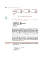
Figure 1.1 Sample word puzzle

because they are entirely impractical for input sizes that a third algorithm can handle in a
reasonable amount of time.
A second problem is to solve a popular word puzzle. The input consists of a twodimensional array of letters and a list of words. The object is to find the words in the puzzle.
These words may be horizontal, vertical, or diagonal in any direction. As an example, the
puzzle shown in Figure 1.1 contains the words this, two, fat, and that. The word this begins
at row 1, column 1, or (1,1), and extends to (1,4); two goes from (1,1) to (3,1); fat goes
from (4,1) to (2,3); and that goes from (4,4) to (1,1).
Again, there are at least two straightforward algorithms that solve the problem. For each
word in the word list, we check each ordered triple (row, column, orientation) for the presence of the word. This amounts to lots of nested for loops but is basically straightforward.
Alternatively, for each ordered quadruple (row, column, orientation, number of characters)
that doesn’t run off an end of the puzzle, we can test whether the word indicated is in the
word list. Again, this amounts to lots of nested for loops. It is possible to save some time
if the maximum number of characters in any word is known.
It is relatively easy to code up either method of solution and solve many of the real-life
puzzles commonly published in magazines. These typically have 16 rows, 16 columns, and
40 or so words. Suppose, however, we consider the variation where only the puzzle board is
given and the word list is essentially an English dictionary. Both of the solutions proposed
require considerable time to solve this problem and therefore might not be acceptable.
However, it is possible, even with a large word list, to solve the problem very quickly.
An important concept is that, in many problems, writing a working program is not
good enough. If the program is to be run on a large data set, then the running time becomes
an issue. Throughout this book we will see how to estimate the running time of a program
for large inputs and, more important, how to compare the running times of two programs
without actually coding them. We will see techniques for drastically improving the speed
of a program and for determining program bottlenecks. These techniques will enable us to
find the section of the code on which to concentrate our optimization efforts.

1.2 Mathematics Review
This section lists some of the basic formulas you need to memorize, or be able to derive,

and reviews basic proof techniques.


1.2 Mathematics Review

1.2.1 Exponents
XA XB = XA+B
XA
= XA−B
XB
(XA )B = XAB
XN + XN = 2XN = X2N
2N + 2N = 2N+1

1.2.2 Logarithms
In computer science, all logarithms are to the base 2 unless specified otherwise.
Definition 1.1

XA = B if and only if logX B = A
Several convenient equalities follow from this definition.
Theorem 1.1

logA B =

logC B
;
logC A

A, B, C > 0, A = 1

Proof

Let X = logC B, Y = logC A, and Z = logA B. Then, by the definition of logarithms, CX = B, CY = A, and AZ = B. Combining these three equalities yields
B = CX = (CY )Z . Therefore, X = YZ, which implies Z = X/Y, proving the theorem.
Theorem 1.2

log AB = log A + log B;

A, B > 0

Proof

Let X = log A, Y = log B, and Z = log AB. Then, assuming the default base of 2,
2X = A, 2Y = B, and 2Z = AB. Combining the last three equalities yields
2X 2Y = AB = 2Z . Therefore, X + Y = Z, which proves the theorem.
Some other useful formulas, which can all be derived in a similar manner, follow.
log A/B = log A − log B
log(AB ) = B log A
log X < X
log 1 = 0,

log 2 = 1,

for all X > 0

log 1,024 = 10,

log 1,048,576 = 20

3

4

Chapter 1

Programming: A General Overview

1.2.3 Series
The easiest formulas to remember are
N

2i = 2N+1 − 1
i=0

and the companion,
N

Ai =
i=0

AN+1 − 1
A−1

In the latter formula, if 0 < A < 1, then
N

Ai ≤
i=0

1
1−A

and as N tends to ∞, the sum approaches 1/(1 − A). These are the “geometric series”
formulas.
i
We can derive the last formula for ∞
i=0 A (0 < A < 1) in the following manner. Let
S be the sum. Then
S = 1 + A + A2 + A3 + A4 + A5 + · · ·
Then
AS = A + A2 + A3 + A4 + A5 + · · ·
If we subtract these two equations (which is permissible only for a convergent series),
virtually all the terms on the right side cancel, leaving
S − AS = 1
which implies that
S=

1
1−A

i
We can use this same technique to compute ∞
i=1 i/2 , a sum that occurs frequently.
We write
2
3
4
5
1

S = + 2 + 3 + 4 + 5 + ···
2 2
2
2
2
and multiply by 2, obtaining

3
2
4
5
6
+
+ 3 + 4 + 5 + ···
2 22
2
2
2
Subtracting these two equations yields
2S = 1 +

S=1+
Thus, S = 2.

1
1
1
1
1
+

+ 3 + 4 + 5 + ···
2 22
2
2
2


1.2 Mathematics Review

Another type of common series in analysis is the arithmetic series. Any such series can
be evaluated from the basic formula:
N

i=
i=1

N(N + 1)
N2
≈
2
2

For instance, to find the sum 2 + 5 + 8 + · · · + (3k − 1), rewrite it as 3(1 + 2 + 3 +
· · · + k) − (1 + 1 + 1 + · · · + 1), which is clearly 3k(k + 1)/2 − k. Another way to remember
this is to add the first and last terms (total 3k + 1), the second and next-to-last terms (total
3k + 1), and so on. Since there are k/2 of these pairs, the total sum is k(3k + 1)/2, which
is the same answer as before.
The next two formulas pop up now and then but are fairly uncommon.
N

i2 =

N3
N(N + 1)(2N + 1)
≈
6
3

ik ≈

Nk+1
|k + 1|

i=1
N
i=1

k = −1

When k = −1, the latter formula is not valid. We then need the following formula,
which is used far more in computer science than in other mathematical disciplines. The
numbers HN are known as the harmonic numbers, and the sum is known as a harmonic
sum. The error in the following approximation tends to γ ≈ 0.57721566, which is known
as Euler’s constant.
N

HN =
i=1

1

≈ loge N
i

These two formulas are just general algebraic manipulations:
N

f(N) = Nf(N)
i=1
N

n0 −1

N

f(i) =
i=n0

f(i) −
i=1

f(i)
i=1

1.2.4 Modular Arithmetic
We say that A is congruent to B modulo N, written A ≡ B (mod N), if N divides
A − B. Intuitively, this means that the remainder is the same when either A or B is
divided by N. Thus, 81 ≡ 61 ≡ 1 (mod 10). As with equality, if A ≡ B (mod N), then
A + C ≡ B + C (mod N) and AD ≡ BD (mod N).

5

6

Chapter 1

Programming: A General Overview

Often, N is a prime number. In that case, there are three important theorems:
First, if N is prime, then ab ≡ 0 (mod N) is true if and only if a ≡ 0 (mod N)
or b ≡ 0 (mod N). In other words, if a prime number N divides a product of two
numbers, it divides at least one of the two numbers.
Second, if N is prime, then the equation ax ≡ 1 (mod N) has a unique solution
(mod N) for all 0 < a < N. This solution, 0 < x < N, is the multiplicative inverse.
Third, if N is prime, then the equation x2 ≡ a (mod N) has either two solutions
(mod N) for all 0 < a < N, or it has no solutions.
There are many theorems that apply to modular arithmetic, and some of them require
extraordinary proofs in number theory. We will use modular arithmetic sparingly, and the
preceding theorems will suffice.

1.2.5 The P Word
The two most common ways of proving statements in data-structure analysis are proof
by induction and proof by contradiction (and occasionally proof by intimidation, used
by professors only). The best way of proving that a theorem is false is by exhibiting a
counterexample.

Proof by Induction
A proof by induction has two standard parts. The first step is proving a base case, that is,
establishing that a theorem is true for some small (usually degenerate) value(s); this step is
almost always trivial. Next, an inductive hypothesis is assumed. Generally this means that

the theorem is assumed to be true for all cases up to some limit k. Using this assumption,
the theorem is then shown to be true for the next value, which is typically k + 1. This
proves the theorem (as long as k is finite).
As an example, we prove that the Fibonacci numbers, F0 = 1, F1 = 1, F2 = 2, F3 = 3,
F4 = 5, . . . , Fi = Fi−1 + Fi−2 , satisfy Fi < (5/3)i , for i ≥ 1. (Some definitions have F0 = 0,
which shifts the series.) To do this, we first verify that the theorem is true for the trivial
cases. It is easy to verify that F1 = 1 < 5/3 and F2 = 2 < 25/9; this proves the basis.
We assume that the theorem is true for i = 1, 2, . . . , k; this is the inductive hypothesis. To
prove the theorem, we need to show that Fk+1 < (5/3)k+1 . We have
Fk+1 = Fk + Fk−1
by the definition, and we can use the inductive hypothesis on the right-hand side,
obtaining
Fk+1 < (5/3)k + (5/3)k−1
< (3/5)(5/3)k+1 + (3/5)2 (5/3)k+1
< (3/5)(5/3)k+1 + (9/25)(5/3)k+1
which simplifies to