Discrete vector fields and the cohomology of certain arithmetic and crystallographic groups
Bạn đang xem bản rút gọn của tài liệu. Xem và tải ngay bản đầy đủ của tài liệu tại đây (1.38 MB, 83 trang )
Discrete vector fields
and the
Cohomology of certain
arithmetic and crystallographic
groups
PhD thesis
by
Bui Anh Tuan
Supervisor: Professor Graham Ellis
School of Mathematics, Statistics and Applied Mathematics
National University of Ireland, Galway
January 2015
Contents
Summary
vi
1 Introduction
1
1.1
Outline of the thesis . . . . . . . . . . . . . . . . . . . . . . . . . . .
2
1.2
Main goals of the thesis
. . . . . . . . . . . . . . . . . . . . . . . . .
2
1.3
Review of necessary background material . . . . . . . . . . . . . . . .
4
1.3.1
CW-spaces . . . . . . . . . . . . . . . . . . . . . . . . . . . . .
4
1.3.2
Cellular chain complexes . . . . . . . . . . . . . . . . . . . . .
7
1.3.3
(Co)homology of groups and ring structure . . . . . . . . . . .
8
2 Vector fields and perturbations
2.1
11
Wall’s technique . . . . . . . . . . . . . . . . . . . . . . . . . . . . . . 12
2.1.1
Proof for theorem 2.0.7 . . . . . . . . . . . . . . . . . . . . . . 14
2.2
Discrete vector fields . . . . . . . . . . . . . . . . . . . . . . . . . . . 16
2.3
Proof of theorem 2.0.6 and related algorithm . . . . . . . . . . . . . . 18
3 Homology of SL2 (Z[1/m])
3.1
24
Resolutions for groups acting on trees . . . . . . . . . . . . . . . . . . 26
i
Contents
3.1.1
3.2
ii
Proof of Theorem 3.1.1 and related algorithms . . . . . . . . . 28
Resolution for SL(2, Z[1/m]) . . . . . . . . . . . . . . . . . . . . . . . 31
3.2.1
Theoretical methods . . . . . . . . . . . . . . . . . . . . . . . 31
3.2.2
Practical results . . . . . . . . . . . . . . . . . . . . . . . . . . 35
4 Crystallographic groups with cubical fundamental domain
4.1
38
Introduction . . . . . . . . . . . . . . . . . . . . . . . . . . . . . . . . 39
4.1.1
Wall’s extension method . . . . . . . . . . . . . . . . . . . . . 41
4.1.2
R¨oder’s method . . . . . . . . . . . . . . . . . . . . . . . . . . 42
4.1.3
Our contribution . . . . . . . . . . . . . . . . . . . . . . . . . 43
4.2
Some definitions . . . . . . . . . . . . . . . . . . . . . . . . . . . . . . 43
4.3
Cubical fundamental domain for crystallographic groups . . . . . . . 46
4.4
Non-free resolutions for crystallographic groups . . . . . . . . . . . . 52
4.4.1
Construction of non-free resolutions . . . . . . . . . . . . . . . 52
4.4.2
Contracting homotopy for cubical case . . . . . . . . . . . . . 55
4.5
Free resolutions for crystallographic groups . . . . . . . . . . . . . . . 56
4.6
Cup product, cohomology ring structure and a proof for Proposition
4.1.1 . . . . . . . . . . . . . . . . . . . . . . . . . . . . . . . . . . . . 57
4.7
Three dimensional Bieberbach groups . . . . . . . . . . . . . . . . . . 58
4.7.1
First group . . . . . . . . . . . . . . . . . . . . . . . . . . . . 59
4.7.2
Second group . . . . . . . . . . . . . . . . . . . . . . . . . . . 60
4.7.3
Third group . . . . . . . . . . . . . . . . . . . . . . . . . . . . 61
4.7.4
Fourth group . . . . . . . . . . . . . . . . . . . . . . . . . . . 62
Contents
iii
4.7.5
Fifth group . . . . . . . . . . . . . . . . . . . . . . . . . . . . 63
4.7.6
Fourth group . . . . . . . . . . . . . . . . . . . . . . . . . . . 65
4.7.7
Sixth group . . . . . . . . . . . . . . . . . . . . . . . . . . . . 66
4.7.8
Seventh group . . . . . . . . . . . . . . . . . . . . . . . . . . . 67
4.7.9
Eighth group . . . . . . . . . . . . . . . . . . . . . . . . . . . 68
4.7.10 Ninth group . . . . . . . . . . . . . . . . . . . . . . . . . . . . 70
4.7.11 Tenth group . . . . . . . . . . . . . . . . . . . . . . . . . . . . 70
4.8
Experimental results . . . . . . . . . . . . . . . . . . . . . . . . . . . 70
4.8.1
Comparison to Wall’s extension method . . . . . . . . . . . . 71
4.8.2
Comparison to R¨oder’s method . . . . . . . . . . . . . . . . . 71
5 Bianchi groups
74
5.1
Reviews of SL(2, O−2 ) . . . . . . . . . . . . . . . . . . . . . . . . . . 75
5.2
H1 (SL(2, O−2 )[1/2], Z) . . . . . . . . . . . . . . . . . . . . . . . . . . 78
5.3
√
−2 . . 79
5.2.1
”non-standard” conjugation with the uniformizer π =
5.2.2
Natural injection . . . . . . . . . . . . . . . . . . . . . . . . . 80
Algorithmetic method for finding a contracting homotopy . . . . . . . 81
Bibliography
83
Summary
This thesis makes the following contributions to the area of Computational Algebraic
Topology:
1. All algorithms written in this thesis are implemented and are publicly available as documented functions for the GAP computer algebra system, and are
distributed with the system as part of the HAP package.
2. We devise and implement an algorithm for computing a finite ZG-equivariant
CW-space with nice cell stabilizer groups and a contracting discrete vector
field, where G = SL2 (Z[1/m]) for any positive integer m. (See Algorithm
3.2.1.)
3. We implement a function which inputs a non-free ZG-resolution and outputs
finitely many terms of a free ZG-resolution R∗G of Z, where G = SL2 (Z[1/m])
for any positive integer m. (See Algorithm 2.1.1.)
4. We devise and implement an algorithm for computing finitely many terms of a
free ZH-resolution R∗H of Z for H a finite index subgroup of G = SL2 (Z[1/m]).
(See Algorithm 3.2.2.)
5. We devise and implement an algorithm that attempts to find a cubical fundamental cell for a cubical crystallographic group G. (See Algorithm 4.3.1).
6. We devise and implement an algorithm that inputs a crystallographic group G
together with a cubical fundamental cell and outputs a finite ZG-equivariant
CW-space with nice cell stabilizer groups and a contracting discrete vector
field. (See Algorithm 4.4.1).
iv
Summary
v
7. We implement a function for calculating finitely many terms of a free ZGresolution R∗G of Z with contracting homotopy, where G is an n-dimensional
cubical crystallographic group. This resolution can be used to compute the
cohomology ring structure of G. (See Algorithm 4.5.1).
8. We devise and implement an algorithm for computing a free ZG-resolution R∗G
of Z with contracting homotopy, where G the full Bianchi group of discriminant
-8, G = SL2 (O−2 ).
9. We provide a cellular complex for the congruence subgroup of level
√
−2 of
the full Bianchi group G = SL2 (O−2 ) in the form of HAP code.
10. We implement a function for calculating a free ZΓ-resolution of Z for Γ the
√
congruence subgroup of level −2 of G = SL2 (O−2 ).
Chapter 1
Introduction
1
1.1 Outline of the thesis
1.1
2
Outline of the thesis
This thesis has seven chapters.
Chapter 1 includes two sections. In the first section we present the main goal of
the thesis, namely methods for calculating the homology of SL(2, Z[1/m]) and the
cohomology ring structure of certain crystallographic groups. The second section
recalls standard material that will be used in the thesis.
Chapter 2 introduces discrete vector fields in the context of group cohomology and
explains how they can be used to find a contracting homotopy on a classifying space.
We also describe a homological perturbation lemma that can be used to construct
a free resolution from a non-free resolution.
Chapter 3 is devoted to constructing a free resolution for SL(2, Z[1/m]) where m is
any positive integer, and calculating the homology of such groups. We describe an
algorithm for computing finitely many terms of a free ZG-resolution of Z for G a
finite index subgroup of SL(2, Z[1/m]. An implementation of the algorithm is used
to determine the integral homology groups Hn (SL(2, Z[1/m]), Z) for all integers
m ≤ 50 (m = 36, 42) , and n ≥ 0.
Chapter 4 provides a method for calculating the cohomology ring structure for Euclidean crystallographic groups with cubical fundamental domain. We describe algorithms for attemping to decide if a given crystallogrpahic group admits a cubical
fundamental domain; and calculating the resulting cellular chain complex as a ZGresolution. We also give a method for computing the contracting homotopy on the
chain complex. Finally we provide a computer method for calculating the cohomology cup product.
1.2
Main goals of the thesis
This thesis has two main topics which are Arithmetic groups and Crystallographic
groups.
1.2 Main goals of the thesis
3
The work on arithmetic groups SL(2, Z[1/m]) was motivated by a question of Kevin
Hutchinson. In his paper [18], Hutchinson stated that he is interested in the precise
structure of H3 (SL2 (Q), Z) and the answer is still unknown. This chapter is written
not to solve Hutchinson’s question but to use it as the motivation since we all know
the class of integral rings Z[1/m] is very close to the field of rational numbers Q as
follows,
Z[1/2] ⊂ Z[1/2.3] ⊂ Z[1/2.3.5] ⊂ · · · ⊂ Z[1/2.3.5...] = Q.
The work is also a generalization of the problem stated in the paper ”On the cohomology of SL(2, Z[1/p])” by A. Adem and N. Naffah [1] in which the authors only
solve the problem for primes p.
The main goal of this part is to present a new method for calculating the group
homology of the arithmetic groups SL(2, Z[1/m]).
Crystallographic groups have been studied for many years and are still an active
topic of research. Some recently published works in the area are [2, 5, 7]. In GAP
[14], we know two methods for calculating the group homology of crystallographic
groups.
One of those two methods is developed and implemented by Graham Ellis, presented
by a function in HAP [9]. His method based on a technique of C.T.C Wall [28]
about group extensions T → G → P . The technique can be applied to a crystallographic group given some methods for computing the free resolutions R∗T and R∗P .
The free ZG-resolution can be constructed by combining those resolutions. This
method works for all crystallographic groups and yields cohomology rings for such
groups. However, for some cases, it produces big ZG-resolutions or doesn’t stop
after one hour of running and some give an error of exceeding permitted memory.
Another method provided by Marc R¨oder [23]. His algorithm uses convex hull computations to construct a fundamental domain for a Bieberbach group and produces
a finite regular CW-space for such a group. The disadvantages are that R¨oder considers only Biebebach groups and uses computational geometry software. Moreover,
for some groups, the fundamental domain produced by this method may have a
complicated shape which we hardly see a accomplishable method to find a contracting homotopy on the cellular chain complexes involving in order to compute the
1.3 Review of necessary background material
4
cohomology rings for such groups.
By seeing the disadvantages of those methods above, we was interested in finding a
new method which could be faster than Ellis and Wall’s and applied to many groups
rather than R¨oder’s. At the time we are writing this thesis, we limit our goal to
the groups that admit a cubical fundamental domain. The reasons are that: we
observe that a high proportion of low-dimensional crystallographic groups admit a
cubical fundamental domain; and we can easily give explicit formula for a contracting homotopy on the cellular chain complex involving. Furthermore, by subdividing
the cubical fundamental domain, we can obtain the Bredon homology which by the
limit of this thesis, we will not mention here.
The main goals of this part are to introduce: (i) new algorithms which attempt to
calculate the group (co)homology of certain crystallographic groups; (ii) a method
for computing the cohomology ring structures for those groups who was successfully
applied in (i).
1.3
Review of necessary background material
This section recalls the basic definitions and concepts needed in the thesis. The
material is standard and taken from [17, 22, 16] with little or no modification.
1.3.1
CW-spaces
This section gives a brief review of CW-spaces. In this thesis, we use the following
notation for the closed unit n-ball , the open unit n-ball and the unit (n − 1)-sphere
Dn = {x ∈ Rn : x ≤ 1},
int(Dn ) = {x ∈ Rn : x < 1},
S n−1 = {x ∈ Rn : x = 1},
where
.
is the standard norm,
(x1 , x2 , . . . , xn ) =
x21 + x22 + . . . + x2n .
1.3 Review of necessary background material
5
Definition 1.3.1. [16] An n-cell is a space homeomorphic to the open n-disk
int(Dn ). A cell is a space which is an n-cell for some n ≥ 0. We say the dimension
of such a cell is n.
Definition 1.3.2. [16] A cell-decomposition (or cell-structure) of a space X is a
family E = {eα |α ∈ I} of subspaces of X such that each eα is a cell and
X=
eα
α∈I
(disjoint union of sets). The n-skeleton of X is the subspace
Xn =
eα
α∈I,dim(eα )≤n
Definition 1.3.3. [16] A pair (X, E) consisting of a Hausdorff space X and a celldecomposition E of X is called a CW-space if the following three axioms are satisfied:
• Axiom 1: (Characteristic Maps) For each n-cell e ∈ E there is a map ϕe :
Dn → X restricting to a homeomorphism ϕe |int(Dn ) : int(Dn ) → e and taking
S n−1 into X n−1 .
• Axiom 2: (Closure Finiteness) For any cell e ∈ E the closure e¯ intersects only
a finite number of other cells in E.
• Axiom 3: (Weak Topology) A subset A ⊆ X is closed iff A ∩ e¯ is closed in X
for each e ∈ E.
The restrictions ϕe |∂Dn are called the attaching maps.
Notice that we can recover X (up to homeomorphism) from a knowledge of X 0 and
the attaching maps. The recovery is described in [17] as follows:
(1) Start with a discrete set X 0 , whose points are regarded as 0-cells.
(2) Inductively, form the n-skeleton X n from X n−1 by attaching n-cells enα via
maps ϕα : S n−1 → X n−1 . This means that X n is the quotient space of the
disjoint union X n−1
α
Dαn of X n−1 with a collection of n-disks Dαn under the
1.3 Review of necessary background material
6
identifications x ∼ ϕα (x) for x ∈ ∂Dαn . Thus as a set X n = X n−1
n
α eα
where
each enα is an open n-cell.
(3) One can either stop this inductive process at a finite stage, setting X = X n
for some n < ∞, or one can continue indefinitely, setting X =
n
X n . In the
latter case X is given the week topology: A set A ⊂ X is open (or closed) iff
A ∩ X n is open (or closed) in X n for each n.
So we have,
X 0 ⊂ X 1 ⊂ X 2 ⊂ ... ⊂ X n ⊂ ...
If there exist an integer n such that X n = X then X is called finite dimensional.
Definition 1.3.4. [17] A CW-space is said to be regular if all its attaching maps
are homemorphisms.
Definition 1.3.5. [15] A map f : X → Y between CW-spaces is cellular if it
satisfies f (X n ) ⊆ Y n for all n.
Definition 1.3.6. [16] A CW-subspace of a CW-space X is a union A of cells in
X such that the closure of each cell is also contained in A; therefore, it is also a
CW-space.
In other words, given a CW-space X =
Y =
α∈I
α∈I
eα and subset I ⊂ I, the union
eα is a CW-subspace of X if e¯α ⊂ Y for all α ∈ I .
Thus X n is a CW-subspace of X, for every n.
Let X be a CW-space and Y be a CW-subspace of X. We say that (X,Y) is a
CW-pair. For an arbitrary CW-space X, we have CW-pairs (X, X n ) for all n and
similarly (X n , X m ) for n ≥ m.
Proposition 1.3.1. [15] Let (X, Y ) be a CW-pair. Then the quotient space X/Y
can be turned in a CW-space such that the quotient map X → X/Y is cellular.
Definition 1.3.7. [17] A G-space is a CW-space together with an action of G on
X which permutes cells. That means, for each g ∈ G a homeomorphism x → gx of
X such that the image gσ of any cell σ is again a cell.
1.3 Review of necessary background material
1.3.2
7
Cellular chain complexes
Let R be a ring. We mainly interested in the integers R = Z and the group ring
R = ZG, where G is a group.
Definition 1.3.8. [29] A chain complex C∗ = (Cn , dn )n∈N of R-modules is a sequence of homomorphisms of R-modules
···
dn+2
/
Cn+1
dn+1
/
Cn
dn
/
Cn−1
dn−1
/
···
d2
/ C1
d1
/
C0
d0
/
0
such that dn dn+1 = 0 for all n. The chain complex C∗ is called an exact sequence if
Im dn+1 = Ker dn for all n.
We say that the chain complex is of length n if Ck = 0 for k > n and Cn = 0. We
refer to the homomorphisms dn as a boundary homomorphisms. The module Ck is
said to be of degree k.
Definition 1.3.9. [29] The k-dimensional homology of a chain complex C∗ over R
is the R−module
Hk (C∗ ) = Ker dk /Im dn+1 .
And the k-dimensional cohomology of C∗ is
H k (C∗ ) = Hk (HomR (C∗ , R))
Suppose that X is a CW-space.
Definition 1.3.10. [17] The cellular chain complex C∗ (X) is the chain complex
that Cn (X) is the free abelian group generated by all n-cells in X
bn
Zeni
Cn (X) =
i=1
where bn is the number of n-cells; and the boundary map can be defined by using
simplicial homology. The definition of the boundary is slightly non-trivial and we
will not described it here. See [17] for the standard definition.
For the purpose of this thesis, we are mainly interested in regular CW-spaces. In
1.3 Review of necessary background material
8
this case, we use a more practical construction for the cellular chain complex based
on the following proposition.
Proposition 1.3.2. [21] Let X be a regular CW-space and let Ck be the free abelian
group formally generated by the k-cells of X. Let dk : Ck → Ck1 be any sequence of
homomorphisms satisfying
(i) dk dk+1 = 0 for any k > 0;
(ii) dk (ekλ ) =
k
k−1
∈X λ,µ eµ
ek−1
µ
k
λ,µ
k
λ,µ
(iii)
where ek−1
ranges over all k − 1-cells of X and
µ
±1
=
0
lies in the boundary of ekλ ,
if ek−1
µ
otherwise;
= [ekλ , ek−1
µ ] is called incident number.
1
1
λ,µ λ,µ
= −1 whenever vertices e0µ , e0µ are incident with a common 1-cell e1λ .
Then the chain complex (C∗ , d∗ ) and the chain complex C∗ (X) of Definition 1.3.10
have isomorphic homology Hn (C∗ ) ∼
= Hn (C∗ ), for n ≥ 0.
Definition 1.3.11. [20] The homology groups of a CW-space X are defined to be
the homology groups of the cellular chain complex C∗ (X).
1.3.3
(Co)homology of groups and ring structure
This section recalls details on homology and cohomology of group via topology. The
main reference of this section is K. S. Brown’s book [4].
Definition 1.3.12. [4] Let R be a ring and M a (left) R-module. A resolution of
M is an exact sequence of R-modules
...
/ F2
∂2
/
F1
∂1
/
F0
/
M
/
0
If each Fi is projective (free), then this is called a projective (free) resolution.
1.3 Review of necessary background material
9
Definition 1.3.13. [4] Let G be a group and ε : F → Z a projective resolution of
Z over ZG, where ZG is the integral group ring of G and Z can be considered as a
ZG-module with trivial G-action. We define the n-th integral homology groups of G
by
Hn (G, Z) = Hn (F ⊗ZG Z)
and the n-th integral cohomology groups of G by
H n (G, Z) = Hn (HomZG (F, Z))
If X is a G-space then the action of G on X induces an action of G on the cellular
chain complex C(X) which thereby becomes a chain complex of G-modules. Moreover, the canonical augmentation
: C0 (X) → Z (defined by (v) = 1 for every
0-cells v of X) is a map of G-modules. In this case, we say that X is a free G-space
if the action of G freely permutes the cells of X. And so that, each chain module
Cn (X) is a free ZG-module with one basis element for every G-orbit of n-cells.
Proposition 1.3.3. [4] Let X be a contractible free G-space. Then the augmented
cellular chain complex of X is a free resolution of Z over ZG.
Proposition 1.3.4. [4] Let X be a free G-space then
C(X/G) ≈ C(X) ⊗ZG Z
Theorem 1.3.5. Let G be a group. If there is a contractible free G-space X then
Hn (G, Z) = Hn (C(X) ⊗ZG Z) = Hn (C(X/G))
and
H n (G, Z) = Hn (HomZG (C(X), Z)) = H n (C(X/G), Z)
Proof for the above theorem comes directly from the Proposition 1.3.3 and Proposition 1.3.4.
The cup product in cohomology is an operation which turns the cohomology groups
of a group G into a graded ring: H ∗ (G, R) =
k≥0
H k (G, R). Details on cup
1.3 Review of necessary background material
10
products can be found in [4]. In this section, we introduce a construction of the cup
product which is implemented in HAP [9].
Definition 1.3.14. [4] Let R∗G be a ZG-resolution of Z. We define that a contracting
G
satisfying
homotopy on R∗G is a family of Z-linear homomorphisms hn : RnG → Rn+1
hn−1 δn + δn+1 hn = 1RnG
for all n ≥ 0 with h−1 = 0 and δ0 = 0.
For any group G there is a bilinear mapping:
H p (G, Z) ⊕ H q (G, Z) → H p+q (G, Z), (u, v) → uv
called the cup product. The product is associative, and uv = (−1)pq vu. The
cup product gives a multiplication on the direct sum of the cohomology groups
H ∗ (G, Z) = ⊕k∈N H k (G, Z). This multiplication turns H ∗ (G; Z) into a ring and now
is called integral cohomology ring of G. The construction of the cup product is as
follows: The cohomology class u ∈ H p (G, Z) is represented by a cocycle u : RpG → Z
G
which induces a chain mapping un : RnG → Rn−p
(for n > p − 1) by recursion using
the contracting homotopy as the diagram below:
G
Rn−p
r
hn−p−1
/
O
q
/
O
un−1
un
/
hn−p−2
G
Rn−p−1
RnG
δn
/
G
Rn−1
G
Rn−p−2
O
un−2
δn−1
/
G
Rn−2
q h1
/
G
R
O 1
s
h0
up+1
G
Rp+1
/
G
R
O 0
−1
s h /
OZ
up
δ1
/
1Z
RpG
u
/Z
The composition of up+q with the cocycle v : RqG → Z is a cocycle representing a
cohomology class uv in Hp+q (G, Z).
Chapter 2
Vector fields and perturbations
11
2.1 Wall’s technique
12
In this chapter, we prove the following useful computational result
Theorem 2.0.6. Let G = SL2 (Z). There is a free ZG-resolution R∗G of Z with
precisely two free generators in each degree greater than 1 and with boundary homomorphism and contracting homotopy explicitly described below.
To prove this theorem we need
(i) a perturbation technique of Wall [28] and
(ii) a discrete vector field on a contractible CW-space X with (non-free) action of
SL2 (Z).
We use Theorem 2.0.6 to obtain an algorithm (Algorithm 2.3.2) that returns the
SL2 (Z)
boundary homomorphism d : R∗
SL2 (Z)
SL2 (Z)
→ R∗
SL2 (Z)
and contracting homotopy h : R∗
R∗
In this chapter we also give a proof for the following theorem in section
Theorem 2.0.7. Let G be a discrete group and X be an n-dimensional regular
contractible G-space such that for each cell σ of X, the stabilizer Gσ fixes σ pointwise.
Suppose that all stabilizer subgroups are contained in a fix periodic group. Then there
is a free periodic ZG-resolution in degree greater than n.
2.1
Wall’s technique
Let G be a discrete group acting on a contractible CW-space X in such a way that the
action permutes cells. Each cell e in X has stabilizer group Ge = {g ∈ G : g.e = e}
whose elements need not stabilize e point-wise. Let [e] denote the equivalence class
of cells in the orbit of e under the action of G, and let Orb(n) denote the set of
equivalence classes of n-dimensional cells. The cellular chain complex C∗ (X) of X
is an exact sequence of ZG-modules with H0 (C∗ (X)) = Z and with
Cp (X) =
[e]∈Orb(p)
ZG ⊗ZGe Ze
→
2.1 Wall’s technique
13
where each Ze is a copy of the integers endowed with an “orientation” action of
Ge . The chain complex C∗ (X) is a ZG-resolution of Z but generally not free. The
method below gives a construction that inputs the non-free ZG-resolution C∗ (X)
together with the free ZGe -resolutions R∗Ge , and outputs a free ZG-resolution R∗G of
Z.
Suppose that for each class [e] we are given a free ZGe -resolution R∗Ge of Z. By
defining
Fp,q :=
[e]∈Orb(p)
ZG ⊗ZGe RqGe
we obtain a free ZG-resolution
Fp,∗ : · · · → Fp,q → · · · → Fp,2 → Fp,1 → Fp,0
of the module Cp (X).
Let
RnG = ⊕p+q=n Fp,q .
(2.1)
Then R∗G is a free ZG-resolution with respects to a differential constructed in the
following propositions:
Proposition 2.1.1. [28] Let Apq p, q ≥ 0 be a bigraded family of free R-modules
for some ring R. Suppose that there are R-homomorphisms d0 : Ap,q → Ap,q−1
such that (Ap,∗ , d0 ) is an acyclic chain complex for each p. Set Cp = H0 (Ap,∗ , d0 )
and suppose further that there are R-homomorphisms δ : Cp → Cp−1 for which
(C∗ , δ) is an acyclic chain complex. Then there exist R-homomorphisms dk : Ap,q →
Ap−k,q+k−1 (k ≥ 1, p > k) such that
(i) di induces δ;
(ii)
k
i=0
di dk−i = 0 for each k (where dk is interpreted as zero if q = k = 0 or if
p < k). Hence d = d0 + d1 + · · · : ⊕p+q=n Apq → ⊕p+q=n−1 Apq is a differential.
Proposition 2.1.2. [28, 10] Let the family of modules A∗,∗ and module homomorphisms d0 : Ap,q → Ap,q−1 and δ : Cp → Cp−1 be as in Proposition 2.1.1. Suppose that
there exist abelian group homomorphisms h0 : Ap,q → Ap,q+1 such that d0 h0 d0 (x) =
d0 (x) for all x ∈ Ap,q+1 . Then we can construct the module homomorphisms dk :
2.1 Wall’s technique
14
Ap,q → Ap−k,q+k−1 and the differential d of Proposition 2.1.1 by first lifting δ to
d1 : Ap,0 → Ap−1,0 and then recursively defining dk = −h0 (
k
i=1
di dk−i ) on free gen-
erators of the module Ap,q . Furthermore, if H0 (C∗ ) ∼
= Z and each Cp is free abelian,
we can construct abelian group homomorphisms h : ⊕p+q=n Ap,q → ⊕p+q=n−1 Ap,q sat-
isfying dhd(x) = d(x) by setting h(ap,q = h0 (a + p, q) − hd+ h0 (ap,q ) + ε(ap,q ) for free
generators ap,q of the abelian group Ap,q . Here d+ =
p
i=1
and, for q ≥ 1, ε = 0.
For q = 0 we define ε = h1 − h0 d+ h1 + hd+ h1 + hd+ h0 d+ h1 where h1 : Ap,0 → Ap+1,0
is an abelian group homomorphism induced by a contracting homotopy on C∗ .
The above construction can be implemented in the form of the following algorithm.
Algorithm 2.1.1 Converting a non-free ZG-resolution to a free ZG-resolution
Input:
• a non-free ZG-resolution C∗ of Z together with free ZGe -resolution of Z for
all stabilizers Ge with contracting homotopy, and
• an integer n ≥ 0.
Output: The first n + 1 terms of a free ZG-resolution R∗G of Z. Moreover, if the
input C∗ is together with a contracting homotopy then the output also together
with a contracting homotopy.
Procedure:
1:
2:
3:
The nth-term RnG is computed by the formula 2.1;
The boundary is constructed by using Proposition 2.1.1;
If the input together with a contracting homotopy then the contracting homotopy of R∗G is constructed by using Proposition 2.1.2.
Algorithm 2.1.1 has already been implemented in HAP package without a contracting homotopy. The contracting homotopy implementation is new and has been done
by the author.
2.1.1
Proof for theorem 2.0.7
Let G be a discrete group and X be an n-dimensional regular contractible G-space.
Let [ei ] denote the equivalence class of i-cells in the orbit of ei under the action of
2.1 Wall’s technique
15
G. The cellular chain complex C∗ (X) of X is
Ci (X) =
[ei ]
ZG ⊗ZGe Z
Suppose that there is a fix group P such that P contains Gei for all i-cells ei ,
0 ≤ i ≤ n. Let R∗P is a free ZP -resolution of Z which is periodic of period m.
Since Gei is a subgroup of P then R∗P can be regarded as a free ZGei -resolution of
Z. Following the construction using Wall’s technique, we have a free ZG-resolution
R∗G . We now prove that RG is periodic in degree greater than n. Since Fp,∗ is the
direct product of periodic resolutions of period m,
Fp,q :=
[e]∈Orb(p)
ZG ⊗ZGe RqGe ,
then Fp,∗ is periodic of period m for all 0 ≤ p ≤ n. That means,
Fp,q = Fp,q+m
(2.2)
for all q > 0. Since the dimension of X is n then Fp,q = 0 for all p > n. Thus,
RkG = ⊕p+q=k Fp,q = ⊕p+q=n Fp,q+k−n
for all k ≥ n. By equation 2.2, then
G
Rk+m
= ⊕p+q=n Fp,q+m+k−n = ⊕p+q=n Fp,q+k−n = RkG .
So that, for all k ≥ n,
G
Rk+m
= RkG
(2.3)
G
We now prove the periodicity of the differential maps d∗ : R∗G → R∗−1
Lemma 2.1.3.
d1p,q = d1p,q+m
where d1p,q : Ap,q → Ap−1,q , for all 1 ≤ p ≤ n and q ≥ 0.
The periodicity of dk : Ap,q → Ap−k,q+k−1 can be obtained by induction starting
2.2 Discrete vector fields
16
from the periodicity of d1 in Lemma 2.1.3.
Assume that the periodicity of dk are proved for all k ≤ N , means that dkp,q = dkp,q+m .
N +1
+1
We will prove that dN
p,q = dp,q+m . By Proposition 2.1.2,
N +1
d
N +1
0
− p, q = −h (
If q = 0 then dN +1 − p, q = −h0 (
N
i=1
di dN +1−i )
i=1
di dN +1−i ). By assumption, di is periodic of
period m for all i ≤ N then
(to be continued)
2.2
Discrete vector fields
In this section we recall the concept of discrete vector field and introduce theoretical
and algorithmic methods to construct a contracting homotopy on a CW-space as an
application of discrete vector field. Material is mainly taken from [13, 12, 24, 19].
Let X be a CW-space, whenever a cell τ ∈ X is attached to a cell σ, we call σ is
a face of τ ; a face of codimension 1 is called a facet. If the attaching map ϕτ of
−1
τ restricts to a homeomorphism on the preimage ϕ−1
τ (σ) and the closure of ϕτ (σ)
is a closed ball, then σ is a regular facet of τ . If all facets are regular then X is a
regular CW-space.
Definition 2.2.1. [13, 24] Consider (C(X), d, β) a cellular chain complex of X
where dn : Cn (X) → Cn−1 (X) is the boundary maps and βn is the cell basis for
Cn (X). If σ k and τ k+1 are respectively a k-cell and (k+1)-cell, then the incidence
number ε(σ k , τ k+1 ) is the coefficient of σ k in the boundary dτ . This incidence number
is non-null if and only if σ k is a face of τ k+1 ; it is ±1 if and only if σ k is a regular
face of τ
Definition 2.2.2. [13, 19] A discrete vector field V on a regular CW-space X is a
collection of arrows s → t where
2.2 Discrete vector fields
17
• s, t are cells and any cell is involved in at most one arrow,
• dim(t) = dim(s) + 1,
• s lies in the boundary of t.
An arrow s → t involves two cells s and t, where s is called the source and t the
target of such arrow. We also write t = V (s) and s = V −1 (t). A cell which is not
involved in any arrow is called a critical cell. A cell basis βn is canonically divided
by the vector field V into three components βn = βnt +βns +βnc where βnt (respectively
βnc , βnc ) is made of the target (respectively source, critical) n-cells.
Definition 2.2.3. [13, 24] Let V be a discrete vector field on CW-space X. Then
a V -path γ of length r from a k-dimensional cell σ k to a k-dimensional cell τ k is a
sequence of arrows ((s0 → t0 ), (s1 → t1 ), . . . , (sr−1 → tr−1 )) ⊂ V satisfying:
• σ k = s0 and τ k in the boundary of tr−1 ,
• si+1 lies in the boundary of ti for all 0 ≤ i < r − 1.
A V-path γ is said to be a cycle if s0 lies in the boundary of tr−1 .
Definition 2.2.4. [13] A discrete vector field is admissible if there is no cycle and
for every source cell s, the length of any path starting from s is bounded by a fixed
integer λ(s), i.e. there is no path of infinite length.
Theorem 2.2.1. [13, 30] If X is a regular CW-space with admissible discrete vector
field then there is a homotopy equivalence
X
Y
where Y is a CW-space whose cells are in one-one correspondence with the critical
cells of X .
Proof of Theorem 2.2.1 can be found in [30] .
We now consider a very special case when the CW-space X is contractible, means
that it can be retracted to a single-point-space. If there is a discrete vector field
describing such a retraction, we shall call it a contracting vector field.
2.3 Proof of theorem 2.0.6 and related algorithm
18
Figure 2.1: DVF on cubical CW-space
Figure 2.1 is an example of a contracting discrete vector field on a 2-dimensional
CW-space with the cubical cell structure.
Theorem 2.2.2. [13, 11, 19] Let C(X) = (C∗ (X), d∗ , β∗ ) be the cellular chain
complex of a contractible CW-space X together with a contracting discrete vector
field V . Then the contracting homotopy on C(X) can be defined as the sum of all
maximal V-paths starting from any n-cell σ n ,
hn (σ n ) =
0
if σ n is not a source
σin+1 ∂n+1 (
σin+1 ) contains just the one
source σ n of dimension n
One can implement this contraction h∗ by using the equivalent recursive formula as
follows:
hn (σ n ) = ε(σ n , V (σ n )) V (σ n ) −
2.3
s −σ n
σ ∈βn
ε(σ , V (σ n ))hn (σ )
Proof of theorem 2.0.6 and related algorithm
Consider the matrices
S=
0 −1
1
0
, T =
1 1
0 1
.
2.3 Proof of theorem 2.0.6 and related algorithm
19
Figure 2.2: Portion of the cubic tree indicated in red
Note that S 4 = (ST )6 = 1 and that the group SL2 (Z) is generated by S and T .
We let M denote the group with presentation s, u | s2 = u3 = 1 . Following [6]
we construct the cubic tree T by taking the left cosets of U = u in M as vertices,
and joining cosets xU and yU by an edge if, and only if, x−1 y ∈ U sU . Thus the
vertex U is joined to sU , usU and u2 sU . The vertices of this tree are in one-to-one
correspondence with all reduced words in s, u and u2 that, apart from the identity,
end in s. We say that a sequence of vertices x0 U , x1 U , . . . , xn U is a rooted path if
x0 = 1 and there is an edge between xi U and xi+1 U for 0 ≤ i ≤ n − 1. A rooted
path is described by a reduced word in s, u and u2 ending in s.
The group M can be realized as the modular group of transformations z → (mz +
n)/(pz + q), m, n, p, q integers with mq − np = 1, of the upper half complex plane
H = {x + iy ∈ C : y > 0} which is generated by the two transformations a(z) =
−1/z and u(z) = z + 1. The cubic tree can thus be embedded in H. Figure 2.2
illustrates this embedding by showing a portion of the cubic tree in bold against
the tessellation of H by triangular fundamental domains for the modular group.
The surjection SL2 (Z) → M, S → s, T → s−1 u and left multiplication in M yield
an action of SL2 (Z) on the cubic tree T . Under this action there is one orbit of
vertices and one orbit of edges. The stabilizer group of any vertex is conjugate to
C6 = ST . The stabilizer group of any edge is conjugate to C4 = S . The cellular
chain complex C∗ (T ) thus has the form
δ
C∗ (T ) : Z[SL2 (Z)] ⊗ZC4 Ze −→ Z[SL2 (Z)] ⊗ZC6 Z
(2.4)
where C6 acts trivially on Z and where Ze denotes the integers with non-trivial action