A SplitPush Approach to 3D Orthogonal Drawing
Bạn đang xem bản rút gọn của tài liệu. Xem và tải ngay bản đầy đủ của tài liệu tại đây (769.05 KB, 29 trang )
Journal of Graph Algorithms and Applications
/>vol. 4, no. 3, pp. 105–133 (2000)
A Split&Push Approach to 3D Orthogonal
Drawing
Giuseppe Di Battista
Maurizio Patrignani
Dipartimento di Informatica e Automazione, Universit`
a di Roma Tre
via della Vasca Navale 79, 00146 Roma, Italy />
Francesco Vargiu
AIPA, via Po 14, 00198 Roma Italy
/>
Abstract
We present a method for constructing orthogonal drawings of graphs
of maximum degree six in three dimensions. The method is based on
generating the final drawing through a sequence of steps, starting from a
“degenerate” drawing. At each step the drawing “splits” into two pieces
and finds a structure more similar to its final version. Also, we test the
effectiveness of our approach by performing an experimental comparison
with several existing algorithms.
Communicated by G. Liotta and S. H. Whitesides: submitted March 1999; revised April 2000.
Research supported in part by the ESPRIT LTR Project no. 20244 - ALCOM-IT
and by the CNR Project “Geometria Computazionale Robusta con Applicazioni alla
Grafica ed al CAD.” An extended abstract of this paper was presented at the 6th
International Symposium on Graph Drawing, GD’98, Montreal, Canada, August 1998.
G. Di Battista et al., 3D Orthogonal Drawing, JGAA, 4(3) 105–133 (2000) 106
1
Introduction
Both for its theoretical appeal and for the high number of potential applications,
research in 3D graph drawing is attracting increasing attention. In fact, low
price high-performance 3D graphic workstations are becoming widely available.
On the other hand the demand of visualization of large graphs increases with
the popularity of the graph drawing methods and tools, and 3D graph drawing
seems to offer interesting perspectives to such a demand. The interest of the 3D
graph drawing community has been mainly devoted to straight-line drawings
and to orthogonal drawings.
Straight-line drawings map vertices to points and edges to straight-line segments. Many different approaches to the construction of straight-line drawings
can be found in the literature. For example, the method presented in [5] distributes the vertices of the graph along a “momentum curve” so that there are
not crossings among the edges. The produced drawings are then “compressed”
into a volume (volume of the smallest box enclosing the drawing) of 4n3 , where
n is the number of vertices of the graph to be drawn. The same paper presents
another algorithm which constructs drawings without edge crossings of planar
graphs with degree at most 4. It “folds” a 2-dimensional orthogonal grid drawing of area h × v into a straight-line drawing with volume h × v.
Another classical approach of the graph drawing field is the force directed
one [7]. It uses a physical analogy, where a graph is seen as a system of bodies
with forces acting among them. These algorithms seek a configuration of the
system with, possibly local, minimal energy. Force directed approaches have
been exploited in 3D graph drawing to devise the algorithms presented in [4, 6,
9, 19, 26, 14, 20].
Further, the research on straight-line drawings stimulated a deep investigation on theoretical bounds. Examples of bounds on the volume of a straight-line
drawing can be found in [5, 21]. Namely, in [5] it is shown that a graph can be
drawn in an n × 2n × 2n volume, which is asymptotically optimal. In [21] it is
shown that, for any fixed r, any r-colorable graph has a drawing with volume
O(n2 ), and that the order of magnitude of this bound cannot be improved.
Special types of straight-line drawings have been studied in [3, 13, 1, 16]
(visibility representations) and in [18] (proximity drawings).
In an orthogonal drawing vertices are mapped to points and edges are
mapped to polygonal chains composed of segments that are parallel to the axes.
Also, it is quite usual to consider a drawing convention in which edges have
no intersections, vertices and bends have integer coordinates, and vertices have
maximum degree six.
Biedl [2] shows a linear time algorithm (in what follows we call it Slices)
that draws a graph in O(n2 ) volume with at most 14 bends per edge. The
drawing is obtained by placing all the vertices on a certain horizontal plane and
by assigning a further horizontal plane to every edge, “one slice per edge”.
Eades, Stirk, and Whitesides [10] propose a O(n3/2 )-time algorithm, based
on augmenting the graph to an Eulerian graph and on applying a variation of an
algorithm by Kolmogorov and Barzdin [17]. The algorithm produces drawings
G. Di Battista et al., 3D Orthogonal Drawing, JGAA, 4(3) 105–133 (2000) 107
that have O(n3/2 ) volume and at most 16 bends per edge. We call this algorithm
Kolmogorov.
The algorithm proposed by Eades, Symvonis, and Whitesides in [11] (we call
it Compact) requires O(n3/2 ) time and volume and introduces at most 7 bends
per edge.
In the same paper [11] Eades, Symvonis, and Whitesides presented a second
algorithm (we call it Three-Bends) whose complexity is linear, while its volume
is 27n3 , and at most 3 bends per edge are introduced. Algorithm Three-Bends is
based on augmenting the graph to a 6-regular graph and on a coloring technique.
The implementation used in the experimental comparison follows the description
of the algorithm given in [11], in which the coloring phase is assumed to run
in O(n3/2 ) time, although in the journal version [12] of the paper [11] Eades,
Symvonis, and Whitesides point out that, by using the result in [25] for the
coloring phase, the actual time complexity of algorithm Three-Bends is O(n).
Papakostas and Tollis [22] present a linear time algorithm (we call it Interactive) that requires at most 4.66n3 volume and at most 3 bends per edge.
It is incremental and can be extended to draw graphs with vertices of arbitrary
degree. The construction starts from a first pair of adjacent vertices, and then
it adds one vertex at a time with its incident edges.
Finally, Wood [28] presents an algorithm for maximum degree 5 graphs that
requires O(n3 ) volume and at most 2 bends per edge. Recently [27], the result
has been extended to maximum degree 6 graphs using no more than 4 bends
per edge. The volume is at most 2.37n3 , the total number of bends is always
less than 7m/3, where m is the number of edges.
Although the results presented in the above papers are interesting and deep,
the research in this field suffers, in our opinion, from a lack of general methodologies.
In this paper we deal with the problem of constructing orthogonal drawings
in three dimensions. Namely, we experiment with several existing algorithms
to test their practical applicability and propose new techniques that have a
good average behavior. Our main target are graphs with vertices in the range
10–100. Such graphs are crucial in several applications [8], like conceptual modeling of databases (Entity-Relationship schemas), information system functions
analysis (Data Flow Diagrams), and software engineering (modules Interaction
Diagrams).
The results presented in this paper can be summarized as follows.
• We present a new method for constructing orthogonal drawings of graphs
of maximum degree six in three dimensions without intersections between
edges. It can be considered more as a general strategy rather than as a
specific algorithm. The approach is based on generating the final drawing
through a sequence of steps, starting from a “degenerate” drawing; at
each step the drawing “splits” into two pieces and finds a structure more
similar to its final version. The new method aims at constructing drawings
without any “privileged” direction and with a routing strategy that is not
decided in advance, but depends on the specific needs of the drawing.
G. Di Battista et al., 3D Orthogonal Drawing, JGAA, 4(3) 105–133 (2000) 108
• We devise an example of an algorithm developed according to the above
method. We call it Reduce-Forks.
• We perform an experimental comparison of algorithms Compact, Interactive, Kolmogorov, Reduce-Forks, Slices, and Three-Bends with a
large test suite of graphs with at most 100 vertices. We measure the
computation time and what we consider to be three important readability
parameters: average volume, average edge length, and average number
of bends along edges. The recent algorithms in [27] and in [12] are not
included in the comparison. Our implementations try to strictly follow
the descriptions given in the papers, without any further improvement.
• Our experiments show that no algorithm can be considered “the best”
with respect to all the parameters. Concerning Reduce-Forks, we can
say that it has the best behavior in terms of the readability parameters
for graphs in the range 5–30, while its effectiveness decreases for larger
graphs. Also, among the algorithms that have a reasonable number of
bends along the edges (Interactive, Reduce-Forks, and Three-Bends),
Reduce-Forks is the one that has the best behavior in terms of edge length
and volume. This is obtained at the expense of an efficiency that is much
worse than the other algorithms. However, the CPU time does not seem
to be a critical issue for the size of graphs in the interval.
The paper is organized as follows. In Section 2 we present our approach
and in Section 3 we argue about its feasibility. In Section 4 we describe Algorithm Reduce-Forks. In Section 5 we present the results of the experimental
comparison.
The interested reader will find at our Web site a CGI program that allows the use of all the algorithms and the test suite used in the experiments
(www.dia.uniroma3.it/∼patrigna/3dcube).
2
A Strategy for Constructing 3D Orthogonal
Drawings
A drawing of a graph represents the vertices as points in 3D space and edges
as curves connecting the points corresponding to the associated vertices. An
orthogonal drawing is such that all the curves representing edges are chains of
segments parallel to the axes. A grid drawing is such that all vertices and bends
along the chains representing the edges have integer coordinates. Further, to
simplify the notation, when this does not cause ambiguities, we shall consider
an orthogonal drawing as a graph with coordinate values for its vertices and
bends.
We also make use of more unusual definitions that describe intermediate
products of our design process. Such definitions allow us to describe “degenerate” drawings where vertices can overlap, edges can intersect, and/or can have
length 0.
G. Di Battista et al., 3D Orthogonal Drawing, JGAA, 4(3) 105–133 (2000) 109
A 01-drawing is an orthogonal grid drawing such that each edge has either
length 0 or length 1 and vertices may overlap. Observe that a 01-drawing does
not have bends along the edges.
A 0-drawing is a (very!) trivial 01-drawing such that each edge has length
0 and all vertices have the same coordinates. A 1-drawing is a 01-drawing such
that all edges have length 1 and vertices have distinct coordinates. (See Fig. 1.)
Observe that while all graphs have a 01-drawing, only some admit a 1-drawing.
For example the triangle graph does not admit a 1-drawing.
Figure 1: A 1-drawing of a graph with ten vertices.
Let G be a graph. A subdivision G1 of G is a graph obtained from G by
replacing some edges of G with simple paths. We partition the vertices of G1 into
vertices that belong also to G (we call them original vertices) and vertices that
belong only to G1 (we call them dummy vertices). Observe that a subdivision
G2 of G1 is a subdivision of G. If G does not have vertices with degree greater
than 6, because of the drawing algorithms mentioned in the introduction, there
always exists a subdivision of G that admits a 1-drawing. From now on, unless
otherwise specified, we deal only with graphs whose maximum degree is at
most 6.
A dummy path of G1 is a path consisting only of dummy vertices except,
possibly, at the endpoints (that can be original vertices). A planar path of an
orthogonal drawing is a maximal path whose vertices are on the same plane. A
planar dummy path is self-intersecting if it has two distinct vertices with the
same coordinates. We consider only paths with at least one edge.
Our method constructs orthogonal grid drawings with all vertices at distinct
coordinates and without intersections between edges (except at the common
endpoints). The drawing process consists of a sequence of steps. Each step maps
a 01-drawing of a graph G into a 01-drawing of a subdivision of G. We start
with a 0-drawing of G and, at the last step, we get a 1-drawing of a subdivision
G1 of G. Hence, an orthogonal grid drawing of G is obtained by replacing each
path of G1 , corresponding to an edge (u, v) of G, with an orthogonal polygonal
G. Di Battista et al., 3D Orthogonal Drawing, JGAA, 4(3) 105–133 (2000) 110
line connecting u and v.
The general strategy is as follows. Let G be a graph. We consider several
subsequent subdivisions of G. We construct an orthogonal grid drawing Γ of G
in four phases.
Vertex Scattering: Construct a scattered representation Γ1 of G, i.e. a 01drawing such that:
• Γ1 is a subdivision of G,
• all the original vertices have different coordinates, and
• all the planar dummy paths are not self-intersecting.
After this phase dummy vertices may still overlap both with dummy and
with original vertices.
Direction Distribution: Construct a direction-consistent representation Γ2
of G, i.e. a 01-drawing such that:
• Γ2 is a scattered representation of G,
• for each vertex v of Γ2 , v and all its adjacent vertices have different
coordinates.
We call this phase Direction Distribution because after this phase the
edges incident on v “leave” v with different directions. Observe that this
is true both in the case v is original and in the case v is dummy.
Vertex-Edge Overlap Removal: Construct a vertex-edge-consistent representation Γ3 of G, i.e. a 01-drawing such that:
• Γ3 is a direction-consistent representation of G,
• for each original vertex v, no dummy vertex has the same coordinates
of v.
After this step the original vertices do not “collide” with dummy vertices.
Observe that groups of dummy vertices sharing the same coordinates may
still exist.
Crossing Removal: Construct a 1-drawing Γ4 that is a vertex-edge-consistent
representation of G.
Observe that, since Γ4 is a 1-drawing, all its vertices, both original and
dummy, have different coordinates. Also, observe that an orthogonal grid
drawing Γ of G is easily obtained from Γ4 .
Each of the above phases is performed by repeatedly applying the same
simple primitive operation called split. Informally, this operation “cuts” the
entire graph with a plane perpendicular to one of the axes. The vertices lying
G. Di Battista et al., 3D Orthogonal Drawing, JGAA, 4(3) 105–133 (2000) 111
in the “cutting” plane are partitioned into two subsets that are “pushed” into
two adjacent planes. A more formal definition follows.
In what follows, the term direction always refers to a direction that is isothetic with respect to one of the axes and the term plane always refers to a
plane perpendicular to one of the axes. Given a direction d we denote by −d
its opposite direction.
Let Γ be a 01-drawing. A split operation has 4 parameters d, P , φ, ρ, where:
• d is a direction.
• P is a plane perpendicular to d.
• Function φ maps each vertex of Γ laying in P to a boolean.
• Function ρ maps each edge (u, v) of Γ laying in P such that φ(u) = φ(v)
and such that u and v have different coordinates to a boolean.
Operation split(d, P, φ, ρ), applied to Γ, performs as follows (see Fig. 2).
1. Move one unit in the d direction all vertices in the open half-space determined by P and d. Such vertices are “pushed” towards d.
2. Move one unit in the d direction each vertex u on P with φ(u) = true.
3. For each edge (u, v) that after the above steps has length greater than
one, replace (u, v) with the new edges (u, w) and (w, v), where w is a new
dummy vertex. Vertex w is positioned as follows.
(a) If the function ρ(u, v) is not defined, then vertex w is simply put in
the middle point of the segment u, v.
(b) Else, (the function ρ(u, v) is defined) suppose, without loss of generality, that φ(u) = true and φ(v) = f alse. Two cases are possible. If
ρ(u, v) = true, then w is put at distance 1 in the d direction from
v. If ρ(u, v) = f alse, then w is put at distance 1 in the −d direction
from u. Roughly speaking, the function ρ is used to specify which is
the orientation of the “elbow” connecting u and v.
Observe that a split operation applied to a 01-drawing of a graph G constructs a 01-drawing of a subdivision of G. Also, although split is a simple
primitive, it has several degrees of freedom, expressed by the split parameters,
whose usage can lead to very different drawing algorithms. Further, split has
to be “handled with care”, since by applying a “random” sequence of split
operations there is no guarantee that the process terminates with a 1-drawing.
G. Di Battista et al., 3D Orthogonal Drawing, JGAA, 4(3) 105–133 (2000) 112
(a)
(b)
Figure 2: An example of split: (a) before the split and (b) after the split.
Vertices with φ = true (φ = f alse) are black (light grey). Edges with ρ = true
(ρ = f alse) are labeled t (f). The little cubes are dummy vertices inserted by
the split.
3
Feasibility of the Approach
In this section we show how the split operation can be used to perform the four
drawing phases described in Section 2.
Since the definition of a scattered representation requires that all the planar
dummy paths are not self-intersecting and since an edge of zero length implies
the existence of a self-intersecting path, we have:
Property 1 All the edges of a scattered representation have length 1.
We now prove that a scattered representation can always be constructed.
Theorem 1 Let Γ0 be a 0-drawing of a graph G. There exists a finite sequence
of split operations that, starting from Γ0 , constructs a scattered representation
of G.
Proof: Consider a sequence of split operations all performed with planes perpendicular to the same axis, say the x-axis, and such that each split separates
one original vertex from the others.
Namely, suppose that the n vertices of Γ0 are labeled v1 , . . . , vn and that all
of them are positioned at the origin. For each i such that 1 ≤ i ≤ n − 1 we
perform split(d, P, φi , ρ) where:
• d is the direction of the x-axis.
G. Di Battista et al., 3D Orthogonal Drawing, JGAA, 4(3) 105–133 (2000) 113
• P is the plane x = 0.
• Function φi maps vertex vi to true and all the other vertices on P to false.
• Function ρ is not defined on any edge.
At the end of the process all vertices lie on the same line and original vertices
have different coordinates. Furthermore, all the obtained dummy paths consist
only of straight line segments with length 1 and with the same direction. Hence,
all dummy paths are not self-intersecting.
✷
Let u be a vertex. We call the six directions around u access directions of
u. Consider the access direction of u determined by traversing edge (u, v) from
u to v; this is the access direction of u used by (u, v). An access direction of u
that is not used by any of its incident edges is a free direction of u.
Given a direction d and a vertex v, we denote by Pd,v the plane through v and
perpendicular to d. The following theorem shows that, starting from a scattered
representation, we can always construct a direction-consistent representation.
Theorem 2 Let Γ1 be a scattered representation of a graph G. There exists a
finite sequence of split operations that, starting from Γ1 constructs a directionconsistent representation of G.
Proof: We consider one by one each vertex u of Γ1 with edges (u, v) and (u, w)
that use the same access direction d of u. Since Γ1 is a scattered representation
of G we have that:
• u is an original vertex, and
• at least one of v and w (say v) is dummy.
Also, by Property 1 we have that all edges incident to u do not have length
0, and hence use a direction of u.
Two cases are possible. Case 1: at least one free direction d of u is orthogonal
to d; see Fig. 3.a. Case 2: direction −d is the only free direction of u; see Fig. 4.a.
Case 1: We perform split(d , Pd ,u , φ, ρ) as follows. We set φ(v) = true, all
the other vertices of Pd ,u have φ = f alse. Also, ρ(u, v) = true, all the other
edges in the domain of ρ have ρ = f alse.
After performing the split (see Figure 3.b), the first edge resulting from the
subdivision of (u, v) uses the direction d of u. The usage of the other access
directions of u is unchanged. Also, all the other vertices still use the same access
directions as before the split with the exception, possibly, of v (that is dummy).
Case 2: Let d be a non-free direction of u different from d. We perform
the same split operation as the one of Case 1, using direction d instead of d .
After the split, (see Figure 4.b), the first edge resulting from the subdivision
of (u, v) uses the direction d of u. At this point, since at least one direction
of the free directions of u is orthogonal to d (direction −d), we can apply the
same strategy of Case 1.
G. Di Battista et al., 3D Orthogonal Drawing, JGAA, 4(3) 105–133 (2000) 114
(a)
(b)
Figure 3: Case 1 in the proof of Theorem 2, before (a) and after (b) the split
operation.
(a)
(b)
Figure 4: Case 2 in the proof of Theorem 2, before (a) and after (b) the split
operation.
Finally, it is easy to observe that the above split operations preserve the
properties of the scattered representations.
✷
In the following we show that, starting from a direction-consistent representation, a vertex-edge-consistent representation can be obtained.
We define a simpler version of split(d, P, φ, ρ), called trivialsplit(d, P ), where
φ is f alse for all vertices of the cutting plane, and, as a consequence, the domain
of ρ is empty. Roughly speaking, trivialsplit has the effect of inserting a new
plane in the drawing that contains only the dummy vertices that are caused
by the edge “stretchings”. We use trivialsplit for tackling the cases where
a dummy vertex has the same coordinates of another vertex. The following
property follows from the definition.
Property 2 Operation trivialsplit does not affect the usage of the access directions of the vertices.
G. Di Battista et al., 3D Orthogonal Drawing, JGAA, 4(3) 105–133 (2000) 115
(a)
(b)
(c)
Figure 5: First case in the proof of Theorem 3.
Theorem 3 Let Γ2 be a direction-consistent representation of a graph G. There
exists a finite sequence of split operations that, starting from Γ2 , constructs a
vertex-edge-consistent representation of G.
Proof: Consider one by one each original vertex u of Γ2 such that there exists
a dummy vertex v with the same coordinates of u. Let (v , v) and (v, v ) be
the incident edges of v. By Property 1 and by the fact that Γ2 is a scattered
representation of G, it follows that v, v and v have different coordinates.
Let d and d be the directions of v used by (v , v) and by (v, v ), respectively (see Fig. 5.a and Fig. 6.a). We perform trivialsplit(d , Pd ,v ) and
trivialsplit(d , Pd ,v ). After performing such operations vertex v is guaranteed
to be adjacent to dummy vertices w and w created by the performed splits.
Two cases are possible (see Fig. 5.b and Fig. 6.b): either d = −d or
not. In the first case we define d as any direction orthogonal to d ; in the
second case we define d as any direction among d , d , and the two directions
orthogonal to d and d . At this point we perform a third split. Namely, we
apply split(d , Pd ,v , φ, ρ) as follows (see Fig. 5.c and Fig. 6.c).
• φ(v) = true, all the other vertices of Pd
,v
have φ = f alse.
• All the edges in the domain of ρ have ρ = true.
Note that at this point u and v have different coordinates. Further, by
Property 2 and because of the structure we have chosen for split we have that the
entire sequence of operations preserves the properties of the direction-consistent
representations, and does not generate new vertex-edge overlaps.
✷
In the remaining part of this section, we study how to perform the last
phase of the general strategy presented in Section 2. Namely, we are going
to show that, given a vertex-edge-consistent representation of a graph G, it
is possible to construct a new vertex-edge-consistent representation of G that
is a 1-drawing. Before introducing the corresponding theorem we need some
intermediate terminology and results.
Let Γ be a 01-drawing of G. We say that two distinct vertex-disjoint planar
paths p and p of Γ on the same plane intersect if there exist two vertices one
G. Di Battista et al., 3D Orthogonal Drawing, JGAA, 4(3) 105–133 (2000) 116
(a)
(b)
(c)
Figure 6: Second case in the proof of Theorem 3.
of p and the other of p with the same coordinates. We denote by χ(Γ) the
number of the pairs of intersecting planar dummy paths of Γ. Observe that
χ(Γ) can be greater than one even if there are just two vertices with the same
coordinates (see Fig. 7).
Figure 7: Two dummy vertices with the same coordinates originating 3 pairs of
intersecting planar dummy paths.
Suppose we need to perform an operation trivialsplit(d, P ) on Γ and let
Γ be the obtained 01-drawing. Let P be the plane of Γ parallel to P and at
distance 1 from P in the d direction.
Property 3 Plane P does not contain any edge of Γ .
Of course this implies that P does not contain any planar path. Also,
because of Property 3, we have:
Property 4 The planar dummy paths of Γ are in one-to-one correspondence
with the planar dummy paths of Γ.
G. Di Battista et al., 3D Orthogonal Drawing, JGAA, 4(3) 105–133 (2000) 117
Property 5 χ(Γ) = χ(Γ ).
Proof: This follows from Property 4 and from the fact that two planar dummy
paths of Γ intersect if and only if the corresponding planar dummy paths of Γ
intersect.
✷
Theorem 4 Let Γ3 be a vertex-edge-consistent representation of a graph G.
There exists a finite sequence of split operations that, starting from Γ3 , constructs a 1-drawing of a subdivision of G.
Proof: Since Γ3 is vertex-edge-consistent, all original vertices have distinct
coordinates, but some dummy vertices may still overlap.
If χ(Γ3 ) = 0, then Γ3 is already a 1-drawing of G. Otherwise, we repeatedly
select a pair of intersecting planar dummy paths p and p (see Fig. 8.a) and “remove” their intersection, decreasing the value of χ. Such removal is performed
as follows.
Let u and v be the end-vertices of p . We have three cases:
1. exactly one of u and v (say v) is an original vertex,
2. both u and v are original vertices, or
3. both u and v are dummy vertices.
In Case 1 (see Figs. 8.a and 8.b) we perform trivialsplit(d, Pd,v ) where d
is the direction p leaves v. In Case 2 we perform trivialsplit(d , Pd ,u ) and
trivialsplit(d , Pd ,v ) where d (d ) is the direction p leaves u (v). In Case 3
we do not perform any trivialsplit.
After the above splits, by Property 5, the value of χ stays unchanged. Also,
observe that the drawing is still a vertex-edge-consistent representation of G.
At this point we concentrate on Case 1, the other cases are similar and are
omitted for brevity. We denote by s the dummy vertex introduced along p by
trivialsplit(d, Pd,v ).
Let d be a direction orthogonal to the plane P where p and p intersect.
We perform split(d , P, φ, ρ), by setting (see Fig. 8.c):
• φ(x) = true for each vertex x ∈ p and x = v, s (f alse otherwise) and
• ρ = true for all the edges in the domain of ρ.
We have that χ decreases after the split by at least one unit. It is easy
to see that such a split preserves the properties of the vertex-edge-consistent
representations.
✷
In this section we have shown that split is a powerful tool in performing the
phases of the strategy presented in Section 2. Namely, each of Vertex Scattering,
Direction Distribution, Vertex-edge Overlap Removal, and Crossing Removal
can be performed by a finite sequence of splits.
G. Di Battista et al., 3D Orthogonal Drawing, JGAA, 4(3) 105–133 (2000) 118
(a)
(b)
(c)
Figure 8: Intersecting planar dummy paths in the proof of Theorem 4. The
black vertex is original. All the other vertices are dummy. The little cubes are
dummy vertices inserted by the split operations described in the proof. Slanted
edges indicate the crossing.
4
The Reduce-Forks Algorithm
Algorithm Reduce-Forks is an example of an algorithm that follows the strategy
described in Sections 2 and 3. Namely, the phases of the strategy are refined into
several heuristics that are illustrated in the following subsections. In Section 5
Reduce-Forks will be compared with the algorithms described in Section 1.
Figs. 9 and 10 show how Reduce-Forks computes a drawing of a K6 graph.
Spheres represent original vertices while cubes represent dummy vertices. Vertices with the same coordinates are drawn inside the same box.
4.1
Vertex Scattering
An edge (u, v) is cut by split(d, P, φ, ρ) if u and v have different values of φ.
Informally, they were in plane P before the split and are in different planes
after the split. A pair of adjacent edges that are cut by a split is a fork.
G. Di Battista et al., 3D Orthogonal Drawing, JGAA, 4(3) 105–133 (2000) 119
(a)
(b)
(c)
(d)
(e)
(f)
Figure 9: The Vertex Scattering phase of algorithm Reduce-Forks applied on
a K6 graph. (a) is a 0-drawing and (f) is a scattered representation.
G. Di Battista et al., 3D Orthogonal Drawing, JGAA, 4(3) 105–133 (2000) 120
(a)
(b)
(c)
(d)
Figure 10: (a–c) the Direction Distribution phase of algorithm Reduce Forks
applied on the scattered representation of the K6 graph of Fig. 9.f (duplicated
in (a) for the convenience of the reader). (d) final drawing. Observe that in this
example the Vertex-edge Overlap Removal and the Crossing Removal phases
are not necessary since (c) is already a 1-drawing.
G. Di Battista et al., 3D Orthogonal Drawing, JGAA, 4(3) 105–133 (2000) 121
Roughly speaking, the heuristic of Reduce-Forks for Vertex Scattering works
as follows. We select an arbitrary pair of original vertices u and v of G with the
same coordinates. Let P , P , and P be the three planes containing u and v.
We consider the set of split operations with planes P , P , and P and that
separate u from v and perform one with “a few” forks. We choose to keep small
the number of forks because each fork will require the insertion of at least one
dummy vertex in the subsequent Direction Distribution phase. Such dummy
vertices will become bends in the final drawing. We repeatedly apply the above
strategy until a scattered representation is obtained.
More formally, observe that finding a split with no forks is equivalent to
finding a matching cut. A matching cut in a graph is a subset of edges that
are pairwise vertex disjoint (matching) and such that their removal makes the
graph disconnected (cut). Unfortunately, the problem of finding a matching cut
in a graph is NP-complete (see [23]). The proof in [23] is based on a reduction
from the NAE3SAT problem [15] and holds for graphs of arbitrary degree.
However, a simple heuristic for finding a cut with a few forks is described
below.
Consider vertices u and v. We color black and red the vertices in the two
sides of the split. Each step of the heuristic colors one vertex. At a certain step
a vertex can be black, red or free (uncolored). At the beginning u is black, v is
red, and all the other vertices are free.
Colored vertices adjacent to free vertices are active vertices. Black (Red)
vertices adjacent to red (black) vertices are boundary vertices. See Fig. 11.
Each step works as follows.
Figure 11: Red, black, and free vertices in the Vertex Scattering heuristic of
Algorithm Reduce-Forks.
1. If a boundary active red vertex, say x, exists, then color red one free
G. Di Battista et al., 3D Orthogonal Drawing, JGAA, 4(3) 105–133 (2000) 122
vertex y adjacent to x. The rationale for this choice is the following: since
vertex x is adjacent to at least one black vertex w (from the definition of
boundary vertex), by coloring y red we prevent a fork between (x, y) and
(x, w). Analogously, if a boundary active black vertex exists, then color
black one of its adjacent free vertices.
2. Else, if an active red vertex, say x, exists, then choose a free vertex y
adjacent to x and color y red. This is done to avoid cutting edge (x, y).
Analogously, if an active black vertex exists, then color black one of its
adjacent free vertices.
3. Else, randomly color black or red a random free vertex.
We perform the above heuristic to each of the subgraphs induced by the
vertices on P , P , and P . Then we select a split with the plane among P ,
P , and P where the cut with the smallest number of forks has been found.
The heuristic can be implemented to run time and space linear in the size
of the current 01-drawing (a graph of maximum degree six has a linear number
of edges).
Observe that, since each split gives different coordinates to at least two
original vertices formerly having the same coordinates, in the worst case the
heuristic is used a number times that is linear in the number of original vertices.
Fig. 9 shows the sequence of splits performed by the heuristic on the K6
graph.
4.2
Direction Distribution
Now, for each original vertex u of G with edges (u, v) and (u, w) such that v and
w have the same coordinates (at least one of v and w is dummy), we have to find
a split that separates v from w (see Fig. 12.a). Of course there are many degrees
of freedom for choosing the split. In Reduce-Forks a heuristic is adopted that
follows the approach of the proof of Theorem 2. However, in performing the
splits we try to move an entire planar dummy path rather than moving a single
dummy vertex. This has the effect of both decreasing the number of bends
(dummy vertices with orthogonal incident edges) introduced by the split, and
of occasionally solving an analogous problem on the other extreme of the planar
dummy path.
More formally, we apply the following algorithm.
1. Compute the (two) planar dummy paths pv and qv containing (u, v) (see
Figs. 12.b–12.c) and the (two) planar dummy paths pw and qw containing
(u, w) (see Figs. 12.d–12.e).
2. For each path of pv , qv , pw , and qw determine the split operations that separate the path (except for the possible original vertices) from all the other
vertices that lie on its plane. For each path we have exactly two possible
splits. Fig. 13 shows the effect of two possible splits on the configuration
of Fig. 12.a.
G. Di Battista et al., 3D Orthogonal Drawing, JGAA, 4(3) 105–133 (2000) 123
(a)
(b)
(c)
(d)
(e)
Figure 12: An example illustrating the heuristic adopted by the Reduce-Forks
algorithm for the Direction Distribution phase. Black vertices are original. All
other vertices are dummy. In (a) two vertices (v, and w) adjacent to the original
vertex u, share the same coordinates. Paths pv , qv , pw , and qw are shown with
dark grey in (b), (c), (d), and (e), respectively.
G. Di Battista et al., 3D Orthogonal Drawing, JGAA, 4(3) 105–133 (2000) 124
(a)
(b)
Figure 13: The effect of applying two different split operations on the configuration shown in Fig. 12.a. In (a) and (b), the planar dummy path pv (Fig. 12.c)
and pw (Fig. 12.e), respectively, is moved in the upward direction by the split.
The split operation corresponding to the latter configuration is preferred by the
Reduce-Forks heuristic since both u and u become direction consistent after
the split.
3. Weight the eight split operations obtained in the previous step according
to the number nd of vertices that become direction-consistent after the
split and, secondarily, to the number of bends they introduce. Observe
that 1 ≤ nd ≤ 2. In the example of Fig. 13 the split described by Fig. 13.b
is preferred to the split described in Fig. 13.a.
4. Select and apply the split operation with minimum weight.
Observe that, since each original vertex requires at most six splits, this
phase is performed with a number of splits that is, in the worst case, linear in
the number of original vertices.
4.3
Vertex-Edge Overlap Removal and Crossing Removal
To perform the Vertex-Edge Overlap Removal and the Crossing Removal phases
a technique is used similar to the one applied for the Direction Distribution
phase. Namely, we identify a set of splits that can “do the job”. We weight
such splits and then apply the ones with minimum weights.
For each original vertex u of G such that v has the same coordinates as u:
1. Compute the (at most three) planar dummy paths containing v.
2. For each path computed in the previous step, determine the split operations that separate the path (except for the possible original vertices)
G. Di Battista et al., 3D Orthogonal Drawing, JGAA, 4(3) 105–133 (2000) 125
from all the vertices that lie on its plane. For each path we have exactly
two possible splits.
3. Weight the split operations obtained in the previous step according to the
number of bends and/or crossings they introduce.
4. Select and apply the split operation with minimum weight.
For each pair of dummy vertices u and v having the same coordinates:
1. Compute all the planar dummy paths containing u or v.
2. Determine all the split operations that separate such paths and u from v.
3. Weight such splits according to the number of bends they introduce.
4. Select and apply the split with minimum weight.
5
Experimental Results
We have implemented and performed an experimental comparison of algorithms
Compact, Interactive, Kolmogorov, Reduce-Forks, Slices, and Three-Bends
with a large test suite of graphs. The experiments have been performed on a
Sun SPARC station Ultra-1 by using the 3DCube [24] system. All the algorithms
have been implemented in C++.
The test suite was composed of 1900 randomly generated graphs having
from 6 to 100 vertices, 20 graphs for each value of vertex cardinality. All graphs
were connected, with maximum vertex degree 6, without multi-edges and selfloops. The density was chosen to be in the middle of the allowed interval: the
number of edges was twice the number of vertices. Note that in a connected
graph of maximum degree 6, the density can range from 1 to 3. Also, as put
in evidence in [8], in the practical applications of graph drawing it is unusual
to have graphs with density greater than 2. The test suite is available at
suite.html
The randomization procedure was very simple. For each graph the number
of vertices and edges was set before the randomization. Edge insertions were
performed on distinct randomized vertices, provided their degree was less than
6 and an edge between the two vertices did not already exist. Non connected
graphs were discarded and re-randomized. The reason for choosing randomized
graphs instead of real-life examples in the tests is that the 3D graph drawing
field, for its novelty, still lacks well established real-life benchmark suites.
We considered two families of quality measures. For the efficiency we relied
on the time performance (CPU seconds); for the readability we measured the
average number of bends along the edges, the average edge length, and the
average volume of the minimum enclosing box with sides isothetic to the axes.
Figs. 14 and 15 illustrate the results of the comparison.
The comparison shows that no algorithm can be considered “the best”.
Namely, some algorithms are more effective in the average number of bends
G. Di Battista et al., 3D Orthogonal Drawing, JGAA, 4(3) 105–133 (2000) 126
(Interactive, Reduce-Forks, and Three-Bends) while other algorithms perform better with respect to the average volume (Compact and Slices) or to the
edge length (Compact, Interactive, and Reduce-Forks). More precisely:
• The average number of bends (see Fig. 14-b) is comparable for Interactive, Reduce-Forks, and Three-Bends, since it remains for all of them
under the value of 3 bends per edge, while it is higher for Compact and
Slices, and it is definitely much too high for Kolmogorov. Furthermore,
Reduce-Forks performs better than the other algorithms for graphs with
number of vertices in the range 5–30. Interactive performs better in the
range 30–100. Another issue concerns the results of the experiments vs.
the theoretical analysis. About Kolmogorov the literature shows an upper
bound of 16 bends per edge [11] while our experiments obtain about 19 on
average. This inconsistency might show a little “flaw” in the theoretical
analysis. Further, about Compact the experiments show that the average
case is much better than the worst case [11].
• Concerning the average edge length (see Fig. 15-a), Reduce-Forks performs better for graphs up to 50 vertices, whereas Compact is better from
50 to 100; Interactive is a bit worse, while the other algorithms form a
separate group with a much worse level of performance.
• The values of volume occupation (see Fig. 15-b) show that Compact and
Slices have the best performance for graphs bigger than 30 vertices, while
Reduce-Forks performs better for smaller graphs.
Examples of the drawings constructed by the experimented algorithms are
shown in Fig. 16.
For these considerations, we can say that Reduce-Forks is the most effective
algorithm for graphs in the range 5–30. Also, among the algorithms that have a
reasonable number of bends along the edges (Interactive, Reduce-Forks, and
Three-Bends), Reduce-Forks is the one that has the best behavior in terms of
edge length and volume. This is obtained at the expense of an efficiency that
is much worse than the other algorithms. However, the CPU time does not
seem to be a critical issue for the size of graphs in this interval. In fact, even
for Reduce-Forks, the CPU time never exceeds 150 seconds, which is still a
reasonable time for most applications.
6
Conclusions and Open Problems
We presented a new approach for constructing orthogonal drawings in three
dimensions of graphs of maximum degree 6, and tested the effectiveness of our
approach by performing an experimental comparison with several existing algorithms.
The presented techniques are easily extensible to obtain drawings of graphs
of arbitrary degree with the following strategy.
G. Di Battista et al., 3D Orthogonal Drawing, JGAA, 4(3) 105–133 (2000) 127
• The Vertex Scattering step remains unchanged.
• In the Direction Distribution step for vertices of degree greater than six, we
first “saturate” the six available directions and then we evenly distribute
the remaining edges.
• The Vertex-edge Overlap Removal step remains unchanged.
• In the Crossing Removal step we distinguish between crossings that are
“needed” because of the overlay between edges that is unavoidable because
of the high degree and the crossings that can be removed. For the latter
type of crossings we apply the techniques presented in Section 3, while
the first type of crossings are handled in a post-processing phase, where
vertices are suitably expanded.
Several problems remain open.
• Devise new algorithms and heuristics (alternative to Reduce-Forks) within
the described paradigm. Such heuristics might be based on modified versions of the 3D graph drawing algorithms listed in Section 1.
• Further explore the trade-offs among edge length, number of bends, and
volume. A contribution in this direction is given by a recent paper by
Eades, Symvonis and Whitesides [12].
• Measure the impact of bend-stretching (or possibly other post-processing
techniques) on the performance of the different algorithms.
• Devise new quality parameters to better study the human perception of
nice drawings in three dimensions.
• Set up test suites, possibly consisting of real-life graphs, specifically devoted to benchmarking 3D graph drawing algorithms.
• Although 3D graph drawing seems to offer interesting perspectives for
the visualization of large graphs, the experiments presented in Section 5
show that the aesthetic quality of the drawings produced with the existing algorithms is still not sufficient to deal with large graphs (see, for
example, Fig. 16). Also in this respect it would be important to improve
the readability of the produced drawings, even at the expenses of a high
computation time.
Acknowledgments
We are grateful to Walter Didimo, Giuseppe Liotta, and Maurizio Pizzonia for
their support and friendship.
G. Di Battista et al., 3D Orthogonal Drawing, JGAA, 4(3) 105–133 (2000) 128
(a)
(b)
Figure 14: Comparison of Algorithms Compact, Interactive, Kolmogorov,
Reduce-Forks, Slices, and Three-Bends with respect to time performance
(a) and average number of bends along edges (b).
G. Di Battista et al., 3D Orthogonal Drawing, JGAA, 4(3) 105–133 (2000) 129
(a)
(b)
Figure 15: Comparison of Algorithms Compact, Interactive, Kolmogorov,
Reduce-Forks, Slices, and Three-Bends with respect to average edge length
(a) and volume occupation (b).