A numerical method for choice of weighting matrices in active controlled structures (p 55 72)
Bạn đang xem bản rút gọn của tài liệu. Xem và tải ngay bản đầy đủ của tài liệu tại đây (278.97 KB, 18 trang )
THE STRUCTURAL DESIGN OF TALL AND SPECIAL BUILDINGS
Struct. Design Tall Spec. Build. 13, 55–72 (2004)
Published online 9 June 2004 in Wiley Interscience (www.interscience.wiley.com). DOI:10.1002/tal.233
A NUMERICAL METHOD FOR CHOICE OF WEIGHTING
MATRICES IN ACTIVE CONTROLLED STRUCTURES
G. AGRANOVICH1, Y. RIBAKOV2,3* AND B. BLOSTOTSKY2
1
Department of Electric Engineering, Faculty of Engineering, College of Judea and Samaria, Ariel, Israel
2
Department of Civil Engineering, Faculty of Engineering, College of Judea and Samaria, Ariel, Israel
3
Institute for Structural Concrete and Building Materials, University of Leipzig, Germany
SUMMARY
A feedback control system usually implements active and semi-active control of seismically excited structures.
The objective of the control system is described by a performance index, including weighting matrix norms. The
choice of weighting matrices is usually based on engineering experience. A new procedure for weighting matrix
components choice based on the parametric optimization method is developed in this study. It represents a twostep optimization process. In the first step a discrete-time control system is synthesized according to a quadratic
performance index. In the second step the weighting coefficients are obtained using the results of the first step.
Numerical simulation of a typical structure subjected to earthquakes is carried out in order to demonstrate the
effectiveness of the proposed method. It shows that applying the proposed technique provides a choice of the
weighting matrices and results in enhanced structural behaviour under different earthquakes. Copyright © 2004
John Wiley & Sons, Ltd.
1.
INTRODUCTION
Active and semi-active damping of seismically excited structures is usually implemented by a feedback control system (Housner et al., 1997; Spencer et al., 1999). The optimal control forces are generally calculated according to the structural behaviour, which is measured during the earthquake and
transferred to a computer. These forces are further produced by actuators or dampers installed in the
structure.
Recent feedback control development methods are based on optimal control theories (Antsaklis and
Mitchel, 1997; Doyle et al., 1989). These methods require the following mathematical description of
the problem. First of all mathematical models of the structure and of the excitation should be obtained.
A performance index for structural behaviour and control rules should then be chosen. The performance index is a measure of the control forces and the regulated variables describing the structural
behaviour. Minimization of this performance index yields an optimal control law.
According to well-known modern approaches the performance index has a form of various matrix
norms, such as L2, H2, and H• (Antsaklis and Mitchel, 1997; Doyle et al., 1989; Spencer et al., 1994;
Dyke et al., 1995). In most practical optimization problems these indices do not directly describe the
problem, because they have no direct physical sense. Indeed, an integral of squared state vector or
control forces vector is very similar to energy. But actually arguing about energy minimization has
again no physical sense, because generally the performance indexes include a sum of such two squares.
The sum yields a compromise between the required and the dissipated energy. However, a reasonable
* Correspondence to: Dr. Ing. Yuri Ribakov, Universitat Leipzig, Marschnerstrasse 31, 04109 Leipzig, Germany. E-mail:
Copyright © 2004 John Wiley & Sons, Ltd.
Received December 2002
Accepted February 2003
56
G. AGRANOVICH ET AL.
question is which energy is ‘more important’ and how it affects the structural response to earthquakes.
Moreover, sometimes an apparent improvement of the performance index leads to a worse structural
response. An additional criterion is proposed in the current study in order to improve the performance
index and to design a control system, providing more efficient control and yielding further decrease
in structural response to earthquakes.
Spencer et al. (1999) described several direct criteria for structural control of seismically excited
buildings. However, the feedback optimal control solutions are known for performance indices in the
form of matrix norms and for linear structural models only. Hence these optimization problems are
commonly employed for structural control optimization.
A classical performance index form is an L2 one with an infinite upper horizon:
•
J (u) = Ú y T (t )Qy(t ) + u T (t ) Ru(t )dt
0
(1)
where y is a vector of structural displacements, velocities and accelerations, u is a control forces vector,
and Q and R are symmetrical non-negative definite weighting matrices describing the balance of the
structural behaviour and of the control action (Dyke et al., 1995; Norgaard et al., 2000).
In any performance index described by Equation (1) the relative magnitudes of the control forces
(components of u) and of the regulated variables (components of y) should also be taken into account.
The matrices Q and R usually have a diagonal form and give different weights to components of
vectors y and u. These weights take into account the different physical nature of the components and
different requirements to their values. Spencer et al. (1999), Dyke et al. (1995), Dyke and Spencer
(1997), Battaini et al. (2000) and others investigated the influence of different weighting coefficients
on the effectiveness of optimum control algorithms applied to earthquake-excited buildings. Generally most of the coefficients are equal to zero. For example, in Dyke and Spencer (1997) only the top
storey acceleration weight is non-zero, whereas in Battaini et al. (2000) only in the two lower storeys
are absolute displacements weights non-zero.
Generally the matrices Q and R are assumed based on practical experience in structural seismic
design. An algorithm for weighting matrix components choice based on parametrical optimization
method is described in this paper.
2.
DESCRIPTION OF THE PROPOSED METHOD
As mentioned above, generally the weighting matrices Q and R selection (Equation 1) is based on
engineering experience. Technical constraints on variables and controls can also be taken into account.
Usually this choice is made by a ‘trial and error’ method. For more qualitative choice of the performance index weighting matrices the following parametrical optimization method is proposed.
The proposed approach is applicable to various weighted performance indices. Its application to
acceleration LQG control design of seismically excited structural control is considered in this study.
The LQG approach is an output feedback design method that has been shown to be effective for design
of acceleration feedback control strategies for this class of systems (Spencer et al., 1994; Dyke et al.,
1995, 1996; Battaini et al., 2000).
Let Jopt be a direct criterion for control strategies evaluation, for example one or several of those
described by Spencer et al. (1999). Thus two criteria are obtained. The first one is J with a known
feedback control solution, and the second one is Jopt, for which the feedback control solution is
unknown. A ‘compromise’ solution is to use the first criterion (J) as a ‘working’ criterion for the second
one (Jopt).
The above-mentioned working criteria contain some weighting parameters. Let these parameters be
defined by W. In this case the second criterion will be a function of weighting parameters W of the
Copyright © 2004 John Wiley & Sons, Ltd.
Struct. Design Tall Spec. Build. 13, 55–72 (2004)
NUMERICAL METHOD FOR CHOICE OF WEIGHTING MATRICES
57
first one, i.e. Jopt(W). For example, for the performance index J described in Equation (1) W collects
the matrices Q and R or their components. Thus the problem is reduced to a choice of W, at which
the optimal control according to criterion J provides a minimum value of the criterion Jopt(W).
This approach enables application of well-developed numerical parametric optimization methods
for solution of the problem described by Nelder and Mead (1965) and Gill et al. (1981). According
to the proposed method, the optimal control synthesis problem should be solved at each step.
The general linear model of the controlled structure according to the proposed optimization method
can be described as follows:
x˙ (t ) = Ac x (t ) + Bc u(kt ) + Ec x˙˙g (t )
(2)
where: x(t) is the state space vector of the system’s continuous part, which includes the vectors of
story displacements and velocities of the structure, and the state vectors of the actuators and the measurement subsystems; u(kt) is the control signal, which is an output signal of a digital controller for
sampling times kt (k = 0, 1, 2, . . .); t is the controller’s sampling period; x˙˙g(t) is the ground acceleration; and the matrices Ac, Bc and Ec describe the continuous part of the whole system. The control
system should be realized in a digital form, hence the differential equations (2) are transformed to an
equivalent system of finite-difference equations (based on an equivalent transformation technique
described in Antsaklis and Mitchel, 1997) as follows:
x (kt ) = Ax (kt ) + Bu(kt ) + Ex˙˙g (kt )
(3)
where
t
t
0
0
A = e Act , B = Ú e Act Bc dt , E = Ú e Act Ec dt
(4)
The output vector contains structural displacements, velocities and accelerations:
y(kt ) = Cx (kt ) + Du(kt ) + Fx˙˙g (kt )
(5)
where matrices C, D and F describe the dependence between the output vector and the structure’s state
vector and excitations.
The measurement vector
ym (kt ) = Cmx (kt ) + Dm u(kt ) + Fm x˙˙g (kt ) + v(kt )
(6)
contains the floor accelerations of the structure. Matrices Cm, Dm and Fm describe the parameters of
the measurement subsystem.
According to the LQG design approach (Dyke et al., 1995, 1996; Battaini et al., 2000) the ground
acceleration x˙˙g(kt) and the measurement noise v(kt) are taken to be a stationary white noise with
known intensity. An infinite horizon performance index (Equation 1) takes in this case the following
form:
J = lim E ÈÍ Â y T (kt )Q1T Q1 y(kt ) + u T (kt ) R1T R1u(kt )˘˙
TÆ• Î
˚
kt £ T
(7)
The square root form of the index weight matrices Q = Q1TQ1 and R = R1TR1 is chosen to avoid the following two problems in parametrical optimization application. The first problem is positive definiteness of index weight matrices constraint, which requires application of much more complicated
Copyright © 2004 John Wiley & Sons, Ltd.
Struct. Design Tall Spec. Build. 13, 55–72 (2004)
58
G. AGRANOVICH ET AL.
parametrical optimization methods with constraints. The second one is the big difference in weight
coefficient values, impairing a convergence property of the parametrical optimization process.
The separation principle allows the control and estimation problems to be considered separately,
yielding a discrete-time dynamic controller (Stengel, 1986). Hence the optimal control law is obtained
as follows:
-1
u(kt ) = - Kxˆ (kt ), K = ( R1T R1 + BT SB) BT SA
(8)
with the same gain matrix as the deterministic LQ2 - control, where S is the solution of the Riccati
algebraic equation given by
-1
A T SA - S - A T SB( R1T R1 + B T SB) B T SA + Q1T Q1 = 0
(9)
A Kalman steady-state estimation xˆ (kt) of the system state vector is obtained from the filter equation:
xˆ (kt + t ) = Axˆ (kt ) + Bu(kt ) + L[ ym (kt ) - Dm u(kt ) - Cm xˆ (kt )]
(10)
where xˆ (kt) is the optimal estimate of the system’s state vector x(kt).
The filter gain matrix L is determined in the following way:
L = ( PCmT + EQm FmT )( Rm + PCmT )
-1
-1
APAT - P + EQm E T + ( PCmT + EQm FmT )( Rm + PCmT ) (Cm P + Fm Qm E T )
(11)
(12)
where Qm and Rm are the intensity matrices of the ground acceleration x˙˙g(kt) and the measurement
noise v(kt) white-noise approximations, respectively.
When the performance index (Equation 7) represents a ‘working’ criterion, Equations (8)–(14) yield
an optimal feedback control LQG optimization problem solution of this index, minimized with linear
dynamic constraints (Equations 3, 5 and 6).
Following Spencer et al. (1999), each proposed control strategy is evaluated for four historical earthquake records: (i) El Centro (California, 1940), (ii) Hachinohe (Hachinohe City, 1968), (iii) Northridge (California, 1994), (iv) Kobe (Hyogo-ken Nanbu, 1995). The appropriate responses have being
used to calculate the evaluation criteria. The evaluation criteria (Spencer et al., 1999) are divided into
four categories: building responses, building damage, control devices, and control strategy requirements. The first three categories have both peak- and norm-based criteria. Small values of the evaluation criteria are generally more desirable. Depending on the purpose and priorities of designing one
of the criteria proposed in Spencer et al. (1999) or their combination, a direct optimization criterion
Jopt can be chosen. As a representative example an optimization problem with a desirable minimum
peak inter-storey drift ratio over the time history of each earthquake is considered:
El Centro ¸
Ï
ÔÔ
di (t ) Hachinohe ÔÔ
J1 = max Ìmax
˝
t ,i
hi Northridge Ô
Ô
ÔÓ
Kobe Ô˛
(13)
under constraints on a peak forces value generated by all the control devices over the time history of
each earthquake:
Copyright © 2004 John Wiley & Sons, Ltd.
Struct. Design Tall Spec. Build. 13, 55–72 (2004)
NUMERICAL METHOD FOR CHOICE OF WEIGHTING MATRICES
El Centro ¸
Ï
ÔÔ
Hachinohe ÔÔ
J11 = max Ìmax ui
˝ £ Umax
t ,i
Northridge Ô
Ô
ÔÓ
Kobe Ô˛
59
(14)
where 0 £ t £ tmax is the time-history earthquake range, 1 £ i £ Nfloors is the building floors range, di(t)
is the inter-storey drift of the above-ground level over the time history of each earthquake, and hi is
the height of the associated storey.
The direct criterion was chosen in the following form:
J opt (W ) = J1 + r( J11 )
(15)
where r(J11) is a penalty function, which possesses zero value if inequality (14) is valid and reaches
a high positive value otherwise. The direct criteria (Equations 13, 14 and 15) calculation for the linear
structure model (Equations 3, 5 and 6) with feedback control (Equations 8 and 10) consists of the following main steps:
(i)
Weighted matrices Q1 and R1 value assignment. Note that all or some of those matrices’ elements
are parameters of the direct optimization criterion Jopt(W).
(ii) Feedback control (Equations 8 and 10) parameters K and L calculation using Equations (8), (9),
(11) and (12).
(iii) Controlled structure simulations over the time history of each earthquake and criteria calculation
using Equations (13), (14) and (15).
An integral optimization algorithm consists of three main blocks (see Figure 1).
Note that the proposed procedure is very similar to a neural net training (Norgaard et al., 2000). In
a similar way the proposed algorithm is based on real excitation data, which is obtained from the historical earthquake records. However, in this case instead of comparison with desired output an optimal
control is realized. It is obvious that for a particular earthquake this control will be optimal if in the
criterion (Equations 13 and 14) only this particular earthquake record is treated. Optimization of the
Structural parameters and initial values
of W0 assignment
Stepwise procedure: Wn + 1 = Wn + s ( Jopt ( Wn ))
and minimum Wopt = arg Min( Jopt ( W )) search
Optimized system simulation and analysis
Figure 1. Parametrical optimization algorithm
Copyright © 2004 John Wiley & Sons, Ltd.
Struct. Design Tall Spec. Build. 13, 55–72 (2004)
60
G. AGRANOVICH ET AL.
criterion (13) yields a control, providing the best structural response to the worst-case earthquake conditions. In contrast to Equation (13) the following modified criterion is used:
J1m
El Centro ¸
Ï
ÔÔ
di (t ) Hachinohe ÔÔ
= Â Ìmax
˝
t ,i
hi Northridge Ô
Ô
ÔÓ
Kobe Ô˛
(16)
It provides the best average result , but not the best structural response to each specific earthquake. In
this case the direct criterion (15) with the above-described penalty function takes the form
J opt (W ) = J1m + r( J11 )
3.
3.1
(17)
NUMERICAL EXAMPLES
Description of the structure and preliminary analysis
In order to demonstrate affectivity and to verify the proposed optimization procedure, MATLAB-based
optimum searches and simulations were carried out. A typical six-storey steel office building (D’Amore
and Astanen-Asl, 1995) designed with UBC-73 (see Figure 2) was chosen for the analysis. The structural system consists of a premier welded MR steel frame (Figure 2). Steel ASTM A36 was used for
all shapes of columns and grids. The stiffness coefficients and floor masses of the building are shown
in Table 1.
The natural frequencies of the chosen structure are 1·083, 2·92, 4·799, 9·596, 7·93 and 6·478 Hz.
An initial damping ratio of 2% was assumed for the first vibration mode of the uncontrolled structure.
columns
beams W24x68
W14x95
400 cm
W24x68
W14x95
400 cm
W24x68
W14x136
400 cm
W24x68
W14x136
400 cm
W24x102
W14x184
400 cm
W24x116
W14x184
520 cm
6 bays × 610 cm
Figure 2. A six-storey structure used for numerical simulation
Copyright © 2004 John Wiley & Sons, Ltd.
Struct. Design Tall Spec. Build. 13, 55–72 (2004)
NUMERICAL METHOD FOR CHOICE OF WEIGHTING MATRICES
61
Table 1. Structural parameters of the six-storey building
Floor number
Floor mass (105 kg)
Stiffness coefficient (105 kg/m)
1·75
1·75
1·75
1·75
1·75
1·75
3·434
0·865
3·009
2·596
2·183
1·092
1
2
3
4
5
6
Table 2. Peak inter-storey drifts of the uncontrolled structure (cm)
Earthquake record
Storey
El Centro
Hachinohe
Northridge
Kobe
4·78
2·11
3·17
2·78
2·95
1·61
3·62
1·41
1·87
1·46
1·72
1·00
7·49
2·83
3·84
3·27
4·32
2·66
15·4
6·59
9·3
7·75
7·95
4·34
1
2
3
4
5
6
Table 3. Peak storey accelerations of the uncontrolled structure (m/s2)
Earthquake record
Storey
El Centro
Hachinohe
Northridge
Kobe
5·2
5·8
6·4
7·7
8·9
10·4
3·2
4·2
5·3
5·2
6·2
8·1
9·6
13·0
14·2
13·8
15·0
18·0
13·8
17·9
20·2
20·5
25·4
30·6
1
2
3
4
5
6
Peak inter-storey drifts and story accelerations of the uncontrolled structure under the selected
earthquakes are given in Tables 2 and 3. These and following numerical results were obtained using
SIMULINK software (MathWorks, 1990) simulation of the structure. To this end a version of the
‘Benchmark simulation program for seismically excited buildings’ (Spencer et al., 1999) modified by
the authors was used. The above-mentioned four earthquake records were considered with single magnitude level (Spencer et al., 1999), which was equal to 1.
Following Spencer et al. (1999) and Battaini et al. (2000) it was assumed that the noised accelerations of all storeys are available and the control actuators are located at each storey of the structure. The dynamics of the measuring instruments and of the control actuators was neglected. Similar
to Spencer et al. (1999), the control force bound Umax in Equation (14) was assumed to be equal to
10,000 N.
Copyright © 2004 John Wiley & Sons, Ltd.
Struct. Design Tall Spec. Build. 13, 55–72 (2004)
62
3.2
G. AGRANOVICH ET AL.
One- and two-parametric optimization
According to the proposed optimization procedure (Figure 1) the vector of optimized parameters W
was chosen. The weight matrices Q1 and R1 of the working performance index J (Equation 7) have
been taken in the following diagonal form:
R1 = I6¥6 , Q1 = diag{qd I6¥6 , qv I6¥6 , qa I6¥6 }
(18)
According to Equation (18) the weights of every control force, inter-storey drifts and storey absolute
velocities have been assumed to be equal to 1, qd and qv, respectively. It should be mentioned that
multiplying the criterion (Equation 7) by a constant does not affect the solution. Thus, only relative
values of the weight parameters are relevant. For this reason the control weights in Equation (18) are
assumed to be equal to one. Note that in the optimization procedures described, for example, in Spencer
et al. (1999), Dyke et al. (1995) and Battaini et al. (2000) it is assumed that qd = qv = 0, but R1 and
Q1 are diagonal matrices with prescribed numerical values. Hence only one optimization parameter qa
is used (one-parameter optimization procedure). Some results of the one-parameter qa optimization
procedure are presented in Tables 4(a–d). In these and the following tables
Table 4(a). Peak inter-storey drifts and storey accelerations of the controlled structure with one-parametric qa
optimization under the El Centro earthquake
Optimization over
El Centro (‘ideal’)
Storey
1
2
3
4
5
6
Optimization according to
(15)
Optimization according to
(17)
Drift (cm)
Acc. (m/s2)
Drift (cm)
Acc. (m/s2)
Drift (cm)
Acc. (m/s2)
1·9
0·7
1·0
0·8
0·8
0·4
4·1
4·7
4·7
4·6
4·3
4·1
1·9
0·7
1·0
0·7
0·8
0·4
4·1
4·7
4·7
4·6
4·2
4·0
1·9
0·7
1·0
0·8
0·8
0·4
4·1
4·7
4·7
4·6
4·2
4·1
P = 606
Control energy
P = 605
P = 605
Table 4(b). Peak inter-storey drifts and storey accelerations of the controlled structure with one-parametric qa
optimization under the Hachinohe earthquake
Optimization over
Hachnohe (‘ideal’)
Storey
1
2
3
4
5
6
Control energy
Optimization according to
(15)
Optimization according to
(17)
Drift (cm)
Acc. (m/s2)
Drift (cm)
Acc. (m/s2)
Drift (cm)
Acc. (m/s2)
1·3
0·5
0·7
0·5
0·5
0·2
1·7
2·2
2·5
2·9
2·9
3·0
1·3
0·6
0·7
0·5
0·5
0·2
1·7
2·2
2·5
2·9
3·0
3·0
1·3
0·5
0·7
0·5
0·5
0·2
1·6
2·2
2·6
2·9
3·0
3·1
P = 352
Copyright © 2004 John Wiley & Sons, Ltd.
P = 352
P = 353
Struct. Design Tall Spec. Build. 13, 55–72 (2004)
63
NUMERICAL METHOD FOR CHOICE OF WEIGHTING MATRICES
Table 4(c). Peak inter-storey drifts and storey accelerations of the controlled structure with one-parametric qa
optimization under the Nothridge earthquake
Optimization over
Nothridge (‘ideal’)
Storey
1
2
3
4
5
6
Optimization according to
(15)
Optimization according to
(17)
Drift (cm)
Acc. (m/s2)
Drift (cm)
Acc. (m/s2)
Drift (cm)
Acc. (m/s2)
6·0
2·4
3·1
2·4
2·3
1·2
88·2
10·0
11·0
11·0
12·0
13·0
6·1
2·1
2·8
2·1
2·0
1·0
8·8
10·0
10·0
10·0
10·0
10·0
6·0
2·1
2·8
2·1
2·0
1·0
8·7
10·0
10·0
10·0
10·0
11·0
P = 1090
Control energy
P = 1470
P = 1450
Table 4(d). Peak inter-storey drifts and storey accelerations of the controlled structure with one-parametric qa
optimization under the Kobe earthquake
Optimization over Kobe
(‘ideal’)
Storey
1
2
3
4
5
6
Control energy
Optimization according to
(15)
Optimization according to
(17)
Drift (cm)
Acc. (m/s2)
Drift (cm)
Acc. (m/s2)
Drift (cm)
Acc. (m/s2)
7·1
2·5
3·3
2·5
2·5
1·2
6·5
7·2
7·0
8·2
8·7
9·1
7·4
2·9
4·0
3·1
3·2
1·6
6·2
7·1
7·8
9·5
11·0
11·0
7·4
3·0
4·1
3·2
3·2
1·6
6·1
7·1
7·9
9·7
11·0
11·0
P = 3800
P = 3770
P=
ÂÚ
1£ i £6
tf
0
xi¢(t ) fi (t ) dt
P = 3780
(19)
is the total energy required for the control of the structure, where fi(t) is the control force developed
by the ith control device and xi¢(t) is the velocity in the ith control device during the earthquake.
First an ‘ideal’ optimization has been performed. A real earthquake record was used as an input
signal. After the parameters of the performance index have been obtained, the same earthquake record
has been applied in order to validate the efficiency of the obtained parameters. The results of this optimization are shown in Tables 4(a–d) (columns 2 and 3).
It is obvious that such optimization is unavailable for application, because it requires prior knowledge of the future earthquake. The ‘ideal’ optimization has been performed for the following two
reasons. First, it enables comparison of the subsequent results of a real optimization with an ‘ideal’
structural behaviour. Secondly, it is possible to show that the values of the optimized parameters essentially depend on the earthquake’s record and not only on the earthquake’s peak ground acceleration
(PGA).
Columns 4 and 5, and 6 and 7, in Tables 4(a–d) present results of one-parametric optimization over
the four chosen earthquakes according to criteria (15) and (17). The weighting coefficient of storey
accelerations qa (Equation 18) was selected as an optimized parameter.
Copyright © 2004 John Wiley & Sons, Ltd.
Struct. Design Tall Spec. Build. 13, 55–72 (2004)
64
G. AGRANOVICH ET AL.
The optimization for each of these two criteria includes about 30–40 steps. Analysis of the optimization process for the criterion (15) shows that for the order of 10–20 steps the process tends to
reduce maximal inter-storey drift under the Kobe earthquake having the highest PGA. After that the
peak inter-storey drift values for the Northridge and Kobe earthquakes are similar. The subsequent
optimization steps tend to provide a compromise between minimum values for these two earthquakes.
The one-parameter optimization is not ideal. Nevertheless for both criteria (15) and (17) and for
each of the four considered earthquakes it yields a close structural response compared to the ‘ideal’
control (Tables 4a–d). However, for the Northridge earthquake it requires higher control energy compared to the ‘ideal’ control.
Tables 5(a–d) present the results of a two-parametric optimization. The weighting coefficients of
inter-storey drifts qd and storey accelerations qa (Equation 18) were selected as optimized parameters.
The process of step optimization for each of two criteria (15 and 17) contains about 50–60 steps
and yields the following results: qd = 7.17 ¥ 107 and qa = 101. Applying two-parametric optimization
yields a decrease in the inter-storey drifts, compared to the one-parametric one; however, it results in
an essential increase of floor accelerations. It should be noted that the addition of a third optimized
parameter qv does not yield any significant improvement compared to the two-parametric optimization results.
Table 5(a). Peak inter-storey drifts and storey accelerations of the controlled structure with two-parametric qd,
qa optimization under the El Centro earthquake
Optimization over
El Centro (‘ideal’)
Storey
1
2
3
4
5
6
Optimization according to
(15)
Optimization according to
(17)
Drift (cm)
Acc. (m/s2)
Drift (cm)
Acc. (m/s2)
Drift (cm)
Acc. (m/s2)
0·7
0·3
0·4
0·3
0·3
0·1
3·2
3·2
4·3
5·3
6·1
6·6
0·7
0·3
0·4
0·3
0·2
0·1
4·5
5·4
7·5
9·2
11·0
11·0
0·7
0·3
0·4
0·3
0·2
0·1
3·3
3·3
4·6
5·6
6·6
7·1
P = 489
Control energy
P = 643
P = 511
Table 5(b). Peak inter-storey drifts and storey accelerations of the controlled structure with two-parametric qd,
qa optimization under the Hachinohe earthquake
Optimization over
Hachnohe (‘ideal’)
Storey
1
2
3
4
5
6
Control energy
Optimization according to
(15)
Optimization according to
(17)
Drift (cm)
Acc. (m/s2)
Drift (cm)
Acc. (m/s2)
Drift (cm)
Acc. (m/s2)
0·6
0·3
0·3
0·2
0·2
0·1
1·5
2·2
3·1
3·9
4·5
4·8
0·6
0·3
0·3
0·2
0·2
0·1
1·1
1·4
2·0
2·4
2·8
3·0
0·6
0·3
0·3
0·2
0·2
0·1
1·0
1·2
1·6
2·0
2·3
2·5
P = 735
Copyright © 2004 John Wiley & Sons, Ltd.
P = 298
P = 269
Struct. Design Tall Spec. Build. 13, 55–72 (2004)
65
NUMERICAL METHOD FOR CHOICE OF WEIGHTING MATRICES
Table 5(c). Peak inter-storey drifts and storey accelerations of the controlled structure with two-parametric qd,
qa optimization under the Nothridge earthquake
Optimization over
Nothridge (‘ideal’)
Storey
1
2
3
4
5
6
Optimization according to
(15)
Optimization according to
(17)
Drift (cm)
Acc. (m/s2)
Drift (cm)
Acc. (m/s2)
Drift (cm)
Acc. (m/s2)
2·8
1·1
1·4
1·0
0·9
0·5
8·0
10
14
16
19
20
2·8
1·1
1·4
1·0
0·9
0·5
8·1
10
14
16
19
20
2·8
1·1
1·4
1·0
0·9
0·5
6·3
6·9
9·2
11
13
14
P = 1640
Control energy
P = 1640
P = 1500
Table 5(d). Peak inter-storey drifts and storey accelerations of the controlled structure with two-parametric qd,
qa optimization under the Kobe earthquake
Optimization over Kobe
(‘ideal’)
Storey
1
2
3
4
5
6
Control energy
Optimization according to
(15)
Optimization according to
(17)
Drift (cm)
Acc. (m/s2)
Drift (cm)
Acc. (m/s2)
Drift (cm)
Acc. (m/s2)
2·0
0·8
0·9
0·7
0·7
0·3
4·2
5·6
7·8
9·3
11
12
2·0
0·8
0·9
0·7
0·7
0·3
3·8
5·1
6·7
8·1
9·2
9·8
2·0
0·8
1·0
0·7
0·7
0·3
3·6
4·6
6·3
7·5
8·7
9·3
P = 2790
P = 2750
P = 2630
Roof displacement and roof acceleration time histories in the uncontrolled structure and in the structure with one- and two-parametric optimization (criterion 17) under the El Centro earthquake are
shown in Figures 3 and 4. The simulation shows that using one-parametric qa optimization yields a
decrease of up to 70% and 60% in roof displacements and accelerations respectively, compared to the
uncontrolled structure. Applying two-parametric qd, qa optimization yields a further essential decrease
in roof displacements compared to one-parametric optimization; however, the accelerations are almost
twice as high as in the uncontrolled structure.
3.3
Six- and twelve-parametric optimization
Supposition regarding the equality of weight matrices’ diagonal elements (Equation 18) used in the
previous numerical example is restrictive. Relaxation of this restriction may lead to further improvement in structural behaviour. Let us assume the weight matrices Q1 and R1 of the working performance index J in Equation (7) have the following form:
R1 = I6¥6 , Q1 = diag{Qd , Qv , Qa }
Copyright © 2004 John Wiley & Sons, Ltd.
(20)
Struct. Design Tall Spec. Build. 13, 55–72 (2004)
66
G. AGRANOVICH ET AL.
Figure 3. Roof displacement time history under the El Centro earthquake (optimization according to
criterion 17)
Figure 4. Roof acceleration time history under the El Centro earthquake (optimization according to
criterion 17)
where Qd, Qv, Qa are diagonal 6 ¥ 6 matrices. Then different weights of every inter-storey drift Qd,
velocity Qv and acceleration Qa are allowed. It is obvious that each of the above-mentioned three
weight matrices include six optimized parameters. Thus, in the examined structure the number of
parameters varies from 6 to 18.
The simulation results of six-parametric optimization for acceleration weights Qa are presented in
Tables 6(a–d). Similar to Spencer et al. (1999), Dyke et al. (1995, 1996), the matrices Qd and Qv have
been assumed to be zero. The optimal parameter values for criterion (15) are
Qa = diag{0◊0007, 0◊0171, 381, 242, 557, 1570}
and for criterion (17) the optimal parameters are
Copyright © 2004 John Wiley & Sons, Ltd.
Struct. Design Tall Spec. Build. 13, 55–72 (2004)
67
NUMERICAL METHOD FOR CHOICE OF WEIGHTING MATRICES
Table 6(a). Peak inter-storey drifts and storey accelerations of the controlled structure with six-parametric Qa
optimization under the El Centro earthquake
Optimization over El
Centro (‘ideal’)
Storey
1
2
3
4
5
6
Optimization according to
(15)
Optimization according to
(17)
Drift (cm)
Acc. (m/s2)
Drift (cm)
Acc. (m/s2)
Drift (cm)
Acc. (m/s2)
1·5
0·6
0·8
0·8
0·7
0·3
3·1
5·2
5·0
4·3
4·0
4·1
1·7
0·6
0·9
0·6
0·7
0·7
3·3
5·4
5·0
5·2
4·5
4·0
1·8
0·6
0·9
0·8
1·3
0·4
3·2
5·4
4·8
4·4
3·7
3·7
P = 683
Control energy
P = 632
P = 640
Table 6(b). Peak inter-storey drifts and storey accelerations of the controlled structure with six-parametric Qa
optimization under the Hachinohe earthquake
Optimization over
Hachinohe (‘ideal’)
Storey
1
2
3
4
5
6
Optimization according to
(15)
Optimization according to
(17)
Drift (cm)
Acc. (m/s2)
Drift (cm)
Acc. (m/s2)
Drift (cm)
Acc. (m/s2)
0·9
0·4
0·5
0·6
0·3
0·4
1·2
2·1
2·0
2·2
2·4
3·1
1·1
0·5
0·6
0·4
0·5
0·4
1·2
2·1
2·5
2·8
2·7
2·5
1·1
0·4
0·6
0·5
0·7
0·3
1·1
2·0
2·2
2·3
2·2
2·2
P = 381
Control energy
P = 346
P = 427
Table 6(c). Peak inter-storey drifts and storey accelerations of the controlled structure with six-parametric Qa
optimization under the Northridge earthquake
Optimization over
Northridge (‘ideal’)
Storey
1
2
3
4
5
6
Control energy
Optimization according to
(15)
Optimization according to
(17)
Drift (cm)
Acc. (m/s2)
Drift (cm)
Acc. (m/s2)
Drift (cm)
Acc. (m/s2)
5·5
2·1
2·8
2·1
2·1
2·2
7
11
11
12
11
9·4
5·4
2·0
2·8
1·9
2·3
1·9
6·8
11
11
12
10
8·7
5·4
1·9
2·8
2·4
3·3
1·2
6·8
11
10
9·4
8·2
8·3
P = 1480
Copyright © 2004 John Wiley & Sons, Ltd.
P = 1620
P = 2270
Struct. Design Tall Spec. Build. 13, 55–72 (2004)
68
G. AGRANOVICH ET AL.
Table 6(d). Peak inter-storey drifts and storey accelerations of the controlled structure with six-parametric Qa
optimization under the Kobe earthquake
Optimization over Kobe
(‘ideal’)
Storey
Optimization according to
(15)
Optimization according to
(17)
Drift (cm)
Acc. (m/s2)
Drift (cm)
Acc. (m/s2)
Drift (cm)
Acc. (m/s2)
3·6
1·3
2·4
3·0
3·0
2·2
3·8
7·5
6·7
6·4
6·7
7·0
6·0
2·4
3·3
2·2
2·8
2·5
3·8
7·8
7·7
8·7
8·6
7·7
4·4
1·7
2·2
2·2
3·3
1·1
3·9
8·2
7·7
7·0
6·5
6·6
1
2
3
4
5
6
P = 3860
Control energy
P = 3920
P = 3810
Qa = diag{19◊8, 0◊0212, 298, 1090, 3480, 3370}
The step optimization process for each of these two criteria includes about 450–550 steps. The results
show the advantage of criterion (17). Peak responses obtained applying this criterion are closer to the
‘ideal’ optimization (columns 4 and 5 and columns 8 and 9 in Tables 6a–d, respectively). However,
the improvement is not significant, and for all the selected earthquakes, except the Kobe one, applying criterion (17) requires higher control energy compared to criterion (15). Applying the sixparametric optimization reduces the higher floor accelerations, compared to the two-parametric
one; however, the inter-storey drifts are higher (Tables 5a–6d).
Finally a twelve-parametric optimization has been carried out. Different weighting coefficients of
inter-storey drift Qd and acceleration Qa were selected as optimized parameters. The process of step
optimization for each of two criteria (15 and 17) contains about 1500–1700 steps and yields the following results:
Qd = diag{1◊25 ¥ 10 7 , 5◊36 ¥ 10 6 , 5◊9 ¥ 10 6 , 18
◊ ¥ 10 8 , 2 ¥ 10 8 , 1 ¥ 10 9 }
Qa = diag{0◊03, 0◊16, 0◊14, 0◊8, 92◊0, 4◊6 ¥ 10 3 }
for criterion (15) and
Qd = diag{4◊67 ¥ 10 6 , 4◊21 ¥ 10 6 , 1◊96 ¥ 10 9 , 5◊02 ¥ 10 8 , 7◊3 ¥ 10 8 , 9◊86 ¥ 10 8 }
Qa = diag{0◊04, 0◊195, 0◊56, 119
◊ , 4◊58, 3◊57 ¥ 10 3 }
for criterion (17).
The peak values of the inter-storey drifts and floor accelerations in the structure with twelveparametric optimization are shown in Tables 7(a–d). Note that applying the twelve-parametric
optimization results in low inter-storey drifts as in case of the two-parametric one and in relatively
low floor accelerations. It is important that for all of the selected earthquakes the required control
energy for the twelve-parametric optimization is the lowest, compared to other cases.
Roof displacement and acceleration time histories of the structure under the El Centro earthquake
for the uncontrolled structure and for the cases of two-, six- and twelve-parametric optimization are
Copyright © 2004 John Wiley & Sons, Ltd.
Struct. Design Tall Spec. Build. 13, 55–72 (2004)
69
NUMERICAL METHOD FOR CHOICE OF WEIGHTING MATRICES
Table 7(a). Peak inter-storey drifts and storey accelerations of the controlled structure with twelve-parametric
Qd, Qa optimization under the El Centro earthquake
Optimization over El
Centro (‘ideal’)
Storey
1
2
3
4
5
6
Optimization according to
(15)
Optimization according to
(17)
Drift (cm)
Acc. (m/s2)
Drift (cm)
Acc. (m/s2)
Drift (cm)
Acc. (m/s2)
0·7
0·3
0·4
0·3
0·2
0·1
4·9
6·2
7·6
9·2
11·0
12·0
0·7
0·3
0·4
0·3
0·2
0·1
5·7
6·8
5·7
4·9
5·2
5·4
0·7
0·4
0·4
0·3
0·2
0·1
13·0
7·4
5·5
4·9
5·2
5·5
P = 647
Control energy
P = 462
P = 511
Table 7(b). Peak inter-storey drifts and storey accelerations of the controlled structure with twelve-parametric
Qd, Qa optimization under the Hachinohe earthquake
Optimization over
Hachinohe (‘ideal’)
Storey
1
2
3
4
5
6
Optimization according to
(15)
Optimization according to
(17)
Drift (cm)
Acc. (m/s2)
Drift (cm)
Acc. (m/s2)
Drift (cm)
Acc. (m/s2)
0·6
0·4
0·3
0·2
0·2
0·1
4·5
2·6
2·6
2·2
2·0
2·0
0·6
0·3
0·4
0·2
0·2
0·1
1·1
1·9
2·0
2·0
1·9
1·9
0·6
0·4
0·3
0·2
0·2
0·1
3·4
2·4
2·3
2·1
1·9
1·9
P = 278
Control energy
P = 246
P = 254
Table 7(c). Peak inter-storey drifts and storey accelerations of the controlled structure with twelve-parametric
Qd, Qa optimization under the Northridge earthquake
Optimization over
Northridge (‘ideal’)
Storey
1
2
3
4
5
6
Control energy
Optimization according to
(15)
Optimization according to
(17)
Drift (cm)
Acc. (m/s2)
Drift (cm)
Acc. (m/s2)
Drift (cm)
Acc. (m/s2)
2·8
1·9
1·3
1·0
0·9
0·5
14·0
8·7
9·1
10·0
11·0
11·0
2·8
1·3
1·6
1·0
0·9
0·5
8·9
11·0
9·7
11·0
11·0
11·0
2·8
1·6
1·3
1·0
0·9
0·5
19·0
10·0
9·5
10·0
11·0
11·0
P = 1500
Copyright © 2004 John Wiley & Sons, Ltd.
P = 1390
P = 1420
Struct. Design Tall Spec. Build. 13, 55–72 (2004)
70
G. AGRANOVICH ET AL.
Table 7(d). Peak inter-storey drifts and storey accelerations of the controlled structure with twelve-parametric
Qd, Qa optimization under the Kobe earthquake
Optimization over Kobe
(‘ideal’)
Storey
1
2
3
4
5
6
Control energy
Optimization according to
(15)
Optimization according to
(17)
Drift (cm)
Acc. (m/s2)
Drift (cm)
Acc. (m/s2)
Drift (cm)
Acc. (m/s2)
2·0
1·5
0·9
0·7
0·6
0·3
7·0
5·4
6·7
7·2
8·2
9·2
2·0
0·9
1·1
0·7
0·6
0·3
4·1
6·1
7·0
7·0
7·8
8·1
2·0
1·1
0·9
0·7
0·6
0·3
11·0
6·4
6·8
7·2
7·6
8·1
P = 2830
P = 2490
P = 2550
Figure 5. Roof displacement time history under the El Centro earthquake (optimization according to criterion
17)
shown in Figures 5 and 6. It demonstrates that applying twelve-parametric optimization yields the
most effective reduction in structural response. Similar results were obtained for the three other
selected earthquakes.
4. CONCLUSIONS
A new procedure for control design of seismically excited structures was developed and verified. The
procedure represents a two-step optimization process. At the first step a discrete-time control system
is synthesized according to a quadratic performance index. At the second step the weighting coefficients for the performance index used in the first one is carried out. It means that the second criterion
is a ‘working’ criterion for the first one.
Numerical simulations of a typical six-storey steel office building were carried out in order to
demonstrate the effectiveness of the proposed optimization procedure. Optimum search and simulaCopyright © 2004 John Wiley & Sons, Ltd.
Struct. Design Tall Spec. Build. 13, 55–72 (2004)
NUMERICAL METHOD FOR CHOICE OF WEIGHTING MATRICES
71
Figure 6. Roof floor acceleration time history under the El Centro earthquake (optimization according to
criterion 17)
tions were carried out by means of MATLAB and SIMULINK-based programs. The numerical simulation showed high efficiency of the proposed method. Its main advantage is providing a choice of
the index weighting coefficients in complicated control problems of multistorey structures, when the
‘trial and error’ method and intuition are ineffective. Applying the proposed algorithm is an efficient
way to further improve the structural response to earthquakes.
Further investigation of the proposed algorithm, including laboratory tests, is required in order to
make it useful for practical applications.
ACKNOWLEDGEMENTS
The Centre of Scientific Absorption of the Ministry of Absorption, State of Israel, supported the
research. The financial support of the Humboldt Foundation, Germany, is greatly appreciated.
REFERENCES
Antsaklis PJ, Mitchel AM. 1997. Linear Systems. McGraw-Hill: New York.
Battaini M, Yang G, Spencer BF Jr. 2000. Bench-scale experiment for structural control. Journal of Engineering
Mechanics, ASCE 126(2): 140–148.
D’Amore E, Astanen-Asl A. 1995. Seismic behavior of six-story instrumented building under 1987 and 1994
Northridge earthquakes. Report No. UCB/CE: Steel 95/03. Department of Civil Engineering, University of
California: Berkeley, CA.
Doyle JC, Glover K, Khargonekar P, Francis B. 1989. State-space solutions to standard H2 and H• control problems. IEEE Transactions on Automatic Control 34: 831–847.
Dyke SJ, Spencer BF Jr. 1997. A comparison of semi-active control strategies for the MR damper. In Proceedings of the IASTED International Conference, Intelligent Information Systems, Bahamas, 8–10 December 1997.
Dyke SJ, Spencer BF Jr, Quast P, Sain MK, Kaspari DC Jr, Soong TT. 1995. Acceleration feedback control of
MDOF structures. Journal of Engineering Mechanics, ASCE 122(9): 897–971.
Dyke SJ, Spencer BF Jr, Quast P, Kaspari DC Jr, Sain MK. 1996. Implementation of active mass driver using
acceleration feedback control. Microcomputers in Civil Engineering, Special Issue on Active and Hybrid Structural Control 11: 305–323.
Gill PE, Murray W, Wright MH. 1981. Practical Optimization. Academic Press: London.
Copyright © 2004 John Wiley & Sons, Ltd.
Struct. Design Tall Spec. Build. 13, 55–72 (2004)
72
G. AGRANOVICH ET AL.
Housner G, Bergman LA, Caughey TK, Chassiakov AG, Claus RO, Masri SF, Skelton RE, Soong TT, Spenser
BF, Yao JTP. 1997. Structural control: past, present, and future. Journal of Engineering Mechanics, ASCE
123(9): 897–971.
MathWorks. 1990. MATLAB User’s Guide. MathWorks: Natick, MA.
Nelder JA, Mead R. 1965. A simplex method for function minimization. Computer Journal 7: 308–313.
Norgaard M, Ravn O, Poulsen NK, Hansen LK. 2000 Neural Networks for Modelling and Control of Dynamic
Systems. Springer: Berlin.
Soong TT. 1990. Active Structural Control: Theory and Practice. Wiley: New York.
Spencer BF Jr, Suhardjo J, Sain MK. 1994. Frequency domain optimal control for aseismic protection. Journal
of Engineering Mechanics, ASCE 120(1): 135–159.
Spencer BF Jr, Christenson RE, Dyke SJ. 1999. Next generation benchmark control problem for seismically
excited buildings. Proceedings of the Second World Conference on Structural Control, Vol. 2. Wiley:
Chichester; 1351–1360.
Stengel RF. 1986. Stochastic Optimal Control: Theory and Application. Wiley: New York.
Copyright © 2004 John Wiley & Sons, Ltd.
Struct. Design Tall Spec. Build. 13, 55–72 (2004)