Srichart 2016-The SEACEN Centre-Determinants of MP transmission via bank lending channel in Thailand-A Threshold Vector Autoregression approach
Bạn đang xem bản rút gọn của tài liệu. Xem và tải ngay bản đầy đủ của tài liệu tại đây (1.55 MB, 30 trang )
Chapter 8
DETERMINANTS OF MONETARY POLICY TRANSMISSION
VIA BANK LENDING CHANNEL IN THAILAND:
A THRESHOLD VECTOR AUTOREGRESSION APPROACH1
By
Kantapon Srichart2
Kongphop Wongkaew3
Suchanan Chunanantatham4
Sukjai Wongwaisiriwat5
1. Introduction
“Most economists would agree that, at least in the short-run,
monetary policy can significantly influence the course of the real
economy...There is far less agreement, however, about exactly how
monetary policy exerts its influence.”
Excerpt from “Inside the Black Box: The Credit Channel of
Monetary Policy Transmission,” Bernanke and Gertler (1995)
We have come a long way toward unraveling the black box on monetary
transmission mechanism. Since the theoretical underpinnings of various channels
have been found, an extensive sum of empirical researches have shed some
light on what happen in the interim from changes in monetary policy to changes
in output and inflation. In light of Thailand experience, the empirical results
point to a transmission mechanism in which banks play an important role,
through the adjustment of both price and quality of loans, relative to
exchange rate and asset price channel. Disyatat and Vongsinsirikul (2002)
argue that the traditional interest rate channel accounts for around half of output
________________
1.
The views expressed in this paper are of the authors and do not reflect those of the Bank
of Thailand, its executives or The SEACEN Centre. All errors and opinions expressed in
this paper are sole responsibility of the authors.
2.
Economist of the Macroeconomic and Monetary Policy Department of the Bank of Thailand.
3.
Economist of the Macroeconomic and Monetary Policy Department of the Bank of Thailand.
4.
Senior Economist of the Macroeconomic and Monetary Policy Department of the Bank
of Thailand.
Economist of the Macroeconomic and Monetary Policy Department of the Bank of Thailand.
5.
233
response after 2 years while Charoenseang and Manakit (2007) show that shocks
to policy rate increase private credits significantly for about 4 month, which in
turn help stimulate output mainly through private investment. Consequently, given
the economy’s heavy reliance on the banking sector, monetary policy effectiveness
is believed to depend largely on commercial banks’ rate adjustment as well as
sensitivity of credits and deposits following changes in policy rate in Thailand.
In a changing economy, the channels of monetary transmission are unlikely
to be constant over time. According to the preliminary studies done for recent
policy easing cycle, the sensitivity of retail rates to money market rates’ reduction
appears to decline, thereby suggesting a weakening interest rate pass-through
after 2010. Meanwhile, monetary easing in Thailand seems to have less influence
in boosting bank loan in the current credit decelerating trend. Therefore, in order
to continuously ensure appropriate design and successful conduct of monetary
policy, it is of great importance to be alerted of the impact of changes that alter
the economic effects of given monetary policy measures. The main objective
of this paper is thus to revisit the transmission via banking sector and identify
the determinants behind those changes for Thai economy.
While there are studies that look into the influences of bank friction on
monetary policy effectiveness both theoretical and empirical6, this paper’s aim
is to test the effect of the boarder economic landscape on monetary policy
effectiveness. Motivated by the current state of economy, we ask whether
monetary policy is effective in an economic downturn period. Intuitively, the
initial economic condition determines where we are on the aggregate supply
curve and how large is the aggregate demand shift as a result of a monetary
policy shock, hence the change in equilibrium output. A shift in aggregate demand
could be larger when the economy is below par and firms are underleveraged
but this trend could be offset by the effect of worsening business confidence.
On the other hand, in an economic downturn phase, when there are large amounts
of spare capacity available, the aggregate supply curve is expected to be very
elastic. Hence, the effect of monetary easing on output is expected to be higher.
With the above hypothesis in mind, we ask whether/how the impact of
monetary policy on macroeconomic dynamics changes with the phase of business
cycle for Thailand. To conduct an empirical exercise, the threshold vector
autoregression (TVAR) methodology is employed as it is appropriate for modeling
regime shifts, i.e., shift between subpar and above par GDP regime. Our results
________________
6. Including Disyatat (2010), Gambarcorta and Marques-Ibanez (2011) and Ananchotikul and
Seneviratne (2015).
234
indicate that the dynamics of the interactions among credit market condition,
economic activities, and monetary policy seems to change as the economy moves
from a subpar growth regime to an above-par regime. Although credit growth
tends to show smaller response to monetary policy easing, possibly due to subdued
private sector confidence, output response seems to be higher during a downturn
when the economy is more likely to be have low capacity utilization.
To set stage for our discussion on monetary policy transmission, we begin
by reviewing the conceptual framework of how transmission channels via banks
could change with the phase of the business cycle in Section 2. Section 3 contains
a brief overview/stylized facts on the transmission mechanism in Thailand. The
methodology and database are presented in Section 4, followed by the empirical
results from the TVAR analysis in Section 5. Section 6 concludes and the
technical details are presented in the appendices.
2. Literature Review and Conceptual Framework
2.1 Conceptual Framework and Theoretical Considerations
Over the past decade, there are a growing number of literatures which
seek to provide evidence that the effectiveness of monetary policy depends,
among other factors, on the state of economic activities. This section provides
a simple framework for investigating the various theories underpinning this
concept. The merit of such a framework is that it allows us to bridge the arguments
which rest on different assumptions and lines of reasoning suggested by each
model with their following empirical results.
According to the traditional macroeconomic concept, the equilibrium of real
output and the price level is determined by the intersection of the aggregate
supply and the aggregate demand curves. Monetary policy affects such
equilibrium, via its influence on aggregate demand. Monetary easing, for instance,
lowers interbank financing costs, and commercial banks typically pass on the
lower cost to their customers in terms of lower lending rates. At the same time,
as funding costs become lower, banks also tend to expand their loan supply. As
a result, private spending and aggregate output rise. Nevertheless, there is
empirical evidence which suggests that loan demand and supply might also depend
on factors other than costs of funds. The following section outlines the key
determinants of loan demand and loan supply respectively. Finally, after
considering the equilibrium in the credit market – which determines the aggregate
demand curve – and the curvature of the aggregate supply curve, we then
move on to explain how monetary policy effectiveness varies with the state of
economic activities.
235
Transmission of monetary policy relies crucially on its role in influencing
credit demand in three ways, as summarized in the following functional form.
Loan demand = f(lending rate, expectation on economic outlook,
borrower’s balance sheet)
Firstly, firms will increase their borrowing if the cost of funds falls below
the internal rate of return. In this sense, the traditional strand of monetary
transmission contends that monetary easing reduces the firm’s cost of fund,
which then induces aggregate demand. However, such a conclusion rests
importantly on the assumption that banks will pass on the lower cost to firms.
Secondly, firms’ demand for borrowing is positively correlated with their
expectation on the outlook of the economy. A bright economic prospect will
prompt firms to acquire more credits to fund their investments. This notion is
supported by Kashyap, Stein, and Wilcox (1993) who provide evidence of a
positive relationship between economic conditions and the demand for bank credit.
Nevertheless, it is important to stress that such a conclusion requires monetary
policy to be sufficiently credible, so that the monetary easing action is perceived
to contribute to a brighter growth prospect going forward. In the absence of
such credibility, the demand for loans may not be as responsive to the monetary
stimulus.
Thirdly, firms’ demand for borrowing is also subject to the prevailing
conditions of their balance sheets. Highly-leveraged firms or firms with
deteriorating balance sheet conditions tend to face limitations in their external
financing. In this respect, monetary easing can alleviate such tensions in their
balance sheets, as a corresponding fall in the discount rate helps increase the
net present value of firms’ assets. The channel in which monetary policy exerts
its influence on firm’s balance sheet is generally referred to as the ‘balance
sheet channel,’ which is one of the two strands of the credit channel of
transmission.
On the supply side, the key factors which determine bank loan supply are
the following:
Loan supply = f(external finance premium, expectation on borrower’s
balance sheet, level of risk aversion)
First of all, the financing condition of a financial intermediary has an influence
on the supply of credit. Monetary policy exerts influence on a bank’s external
236
funding cost by directly setting the policy rate, which in turn acts as short-term
benchmark rates in the financial markets. At the same time, monetary policy
influences market expectation of future path of interest rate, which then affects
the costs of longer-term financing. In addition, monetary easing indirectly affects
the default risk premium which banks face in tapping market financing due to
its influence on banks’ balance sheets. Monetary easing which pump up asset
prices also improve banks’ net worth in the same way as the effects of the
aforementioned effects on firms’ balance sheet.
Firms’ balance sheets also play a role in determining the provision of credit.
Bernanke and Gertler (1989) designed a model of business cycle with the
inclusion of the role of firms’ balance sheets for highlighting this concept.
Assuming that a bank maximizes profit and has to deal with imperfect information
of the borrowers, the expected net worth of a firm serves as a leading indicator
of a borrower’s probability to default. As a firm’s wealth deteriorates, adding
to the possibility of a default, a bank may guard its wealth against such default
risks by tightening the credit condition and vice-versa. The key implication is
that this mechanism becomes a source of pro-cyclicality, exacerbating the
downturn and fueling the expansion. Bayoumi and Melander (2008) developed
the macrofinancial linkages and found significant evidence that credit conditions
have influence on real spending.
Finally, loan supply may also vary with risk aversion of financial intermediaries
which changes in response to business/economic outlook. Kahneman and Tversky
(1979) proposed the so-called prospect theory which argues that when economic
agents become risk averse in an environment, consumption will fall below a
habit-based reference level – a concept which could also help explain the behavior
of banks. The implication is that an economic recession usually concurs with
some sort of confidence crisis, which further acts as a propagator of negative
shocks to economic growth, delaying the recovery.
Putting together the factors affecting loan demand and supply would result
in the equilibrium in the loan market. This, in turn, determines the magnitude of
the shift in the aggregate demand curve following a monetary easing action. In
the low-growth regime, for instance, if the sentiment factor dominates a fall in
financing costs, then a shift in aggregate demand (AD) will be marginal.
However, in the absence of negative sentiment or uncertainty, a shift in AD will
be relatively larger.
The shape of the aggregate supply curve also plays a role in determining
the effectiveness of monetary policy. Keynes is among the earlier supporters of
237
this argument which suggests that the aggregate supply (AS) curve is positivelysloped up to the expected price level and vertical afterwards as the economy
reaches its long-run potential. The Keynesian concept implies that monetary
policy shocks in the state of high economic activity are neutral but those in a
low-activity environment are effective, implying that monetary policy is more
powerful in a state of low economic growth than in the period of expansion.
Related theories include the ‘costly price adjustment’ strand, cited in Tsiddon
(1993), and Ball and Mankiw (1994). Ball and Mankiw (1994) proposed the socalled “Menu Cost” model which is derived on microeconomic foundations. The
model assumes that a single firm bears “the Menu Cost” of adjusting prices to
maintain the relative price of its goods to the overall price, in a backdrop of
continuing positive inflation. The authors argue that a positive inflation rate helps
offset a negative shock in overall prices, bringing the relative price back to its
preferable level without needing any downward adjustment. On the contrary,
inflation acts as propagator of positive shock to the overall price and the firm
has to raise its price even higher to shore up its relative price towards the
desired level. Thus, a firm is more likely to adjust their price upwards rather
than downwards, with implications of a convex aggregate supply curve.
Based on this simple AD-AS framework, the resulting equilibrium output
depends on two forces – the magnitude of shift in the AD curve, and the slope
of the AS curve. For instance, in a state of high economic activity, a monetary
easing shock may shift AD significantly, but given the relatively steep AS curve,
the effect on output would become smaller.
2.2 Empirical Evidence
2.2.1
Reviews of Literatures on Monetary Policy Transmission in
Thailand
Literatures on transmission via the banking sector in Thailand are divided
into two main strands. The first strand of research concerns the quantitative
assessment of the consequences of a change in the policy rate on macroeconomic
variables and how they change over time. The second strand focuses on the
determinants of the transmission mechanism. Finally, we also outline the key
factors underlying the evolution of monetary transmission in the past decade.
Regarding traditional interest rate channel, the prominent view is that there
was a significant decline in the pass-through from the policy rate to bank retail
rates in Thailand following the East Asian financial crisis in 1997. Using the
238
Error Correction Model (ECM) analysis, Disyatat and Vongsinsirikul (2002) argued
that the retail rates in Thailand is generally sticky to policy rate movement
compared to those in developed countries and they became stickier in the
aftermath of the crisis. These results are consistent with Atchana and Singhachai
(2008), whose work documents a decline in the responsiveness of retail rates
to policy rate changes following the financial crisis, with stickiness of policy
pass-through being most evident around 2004-2005. Also, Charoenseang and
Manakit (2007) found that despite the observable long-run relationship between
the policy rate and money market rates, the pass-through effect of the policy
rate on banks’ retail rates is quite low, at about 20% during 2000-2006. The
authors also estimated the vector autoregression (VAR) system on Thailand
data during 2000-2006 and found that the policy rate does not strongly influence
the lending rate, suggesting a weaker transmission through interest rate channel
after the adoption of inflation targeting in 2000.
According to the abovementioned literatures, level of competition and the
liquidity in the banking sector are noted as the two main catalysts. Disyatat and
Vongsinsirikul (2002) contend that a cost of rate adjustment is higher in the less
competitive banking sector than in a more competitive system. In addition Atchana
and Singhachai (2008) argue that the degree of risk aversion in the banking
system has changed since the outbreak of the 1997 financial crisis, as bank
reserves greater portion of cash and liquid assets in excess of the legal
requirement. Against this backdrop, marginal tightening in monetary policy would
not be able to tempt banks to raise its lending rates. Charoenseang and Manakit
(2007) draw a similar conclusion on excess liquidity. It was not until mid-2015
that the excess liquidity started to reduce, after which the interest rate passthrough began to pick up more evidently.
Most of the literatures on monetary transmission generally agree that the
bank lending channel could help amplify the effect of interest rate shock beyond
what would be predicted if the monetary policy were to transmit its effect through
the interest rate channel alone. According to Disyatat and Vongsinsirikul (2002),
monetary tightening leads to a fall in bank credits with about 3 quarters lag and
bank loans also have significant implication on the impulse response of GDP
from interest rate shocks. Similarly, Charoenseang and Manakit (2007) found
that shocks to monetary policy induced major changes in commercial banks
credits to private sector for about 4 months while commercial bank credits have
strong impact on private investment.
However, there is a growing recognition that the significance of the credit
channel and the importance of bank loans have declined since the crisis period.
239
As argued by Disyatat and Vongsinsirikul (2002), the sensitivity of loan supply
to monetary shocks has gone down since 1999, along with effectiveness of
monetary policy associated with the bank lending channel. By comparing the
VAR of the whole sample and truncated data of up to 1999, the paper finds that
the response of output and bank credits to monetary policy of a similar size is
more pronounced in the pre-crisis period. The authors argued that this is attributed
to a rise in prominence of non-deposit funding for banks, which serve as a
cushion against a tightening of monetary policy, in turn reducing the sensitivity
of loan supply and output to monetary shocks. Also, a firm can substitute nonbank
financing for bank loans when monetary policy tightens.
In addition, Disyatat and Vongsinsirikul (2002) also focused on the financial
health of the banking and corporate sector which affects how monetary shock
is translated into bank credit, the chief motivation of our study. By effectively
constraining new bank lending, a continued weakness in the banking sector
following the crisis, tended to offset the impact of monetary easing. At the same
time, excess capacity and balance sheet weakness in the corporate sector also
act as a constraint on investment demand, thereby blunting the credit channel
of monetary policy. We will elaborate more on this argument.
Nonetheless, there are also a few literatures, providing evidences in favor
of an improved bank lending channel. Amarase and Rungcharoenkitkul (2014)
offers a model to support the fact that greater bank competition and lower riskfree rate raise the screening costs, eventually leading to a pooling equilibrium
involving larger credits at cheaper prices. In context of the Thai experience, a
shift in Specialized Financial Institutions’ (SFIs) lending strategy may have
triggered a transition of equilibrium from credit rationing to credit boom. As
competition and risk-taking intensified during the 2011-2013 easing episode, banks
strategically increased credit supply, as reflected by a compressed spread.
Therefore, bank competition can play an important part in strengthening the
impact of monetary policy on bank lending and economy during the current
easing cycle.
In sum, based on literature of the Thai experience, banks are still central
elements in monetary policy transmission mechanism. Nevertheless, its relevance
has declined mainly through the price perspective. On top of the monetary policy
framework which should influence the degree of transmission, the literature also
point to (i) excess liquidity and competition in banking sector; (ii) financial
deepening; and, (iii) financial health of banks.
240
2.2.2
Evidence of Non-linear Monetary Policy Influence on Real
Output
Many literatures confirm the non-linear interaction between monetary policy
and real output with regard to a state of economy. In the case of developed
countries, the earlier study of Garcia and Schaller (2002) examined the goodness
of fit of the Markov-switching model which treats the state of economy as a
latent variable versus the linear model in simulating the response of output to
policy rate. Their results confirm the existence of the asymmetry regarding the
economic environment. Lo and Piger (2003) also deploy VAR analysis on the
US data during 1954Q3 to 2002Q4 and find strong evidence of time variation
in the relationship between monetary policy and output. Regressing the
probabilities of change in this relationship on several state variables, the authors
find strong evidence that regime shifts can be well explained by the phase of
the business cycle. The study, however, finds no strong evidence in favor of
asymmetry with regard to the direction of policy action and does not test whether
policy direction matters within each growth regime. Some of the literatures adopt
the threshold vector autoregression (TVAR) model, including Balke (2000) who
tested the two-regime switching model and Avdjiev and Zeng (2014) who
developed a three-regime switching model in similar spirit to Balke (2000). Both
studies corroborate the existence of the asymmetry. Other papers include Weise
(1999), and Thoma (1994).
Using U.S. data, empirical literatures show mixed results. The first group
favors the argument for more potent monetary policy in a state of low-economic
growth than those in high growth periods, namely Weise (1999), Balke (2000),
Garcia and Schaller (2002), and Lo and Piger (2003) and Avdjiev and Zeng
(2014). Estimations deployed in Garcia and Schaller (2002) affirms that the effect
of monetary tightening on output is more powerful during recessions than during
expansions.
According to the credit-rationing proposition, Balke (2000) finds that monetary
tightening shocks are more potent in the tight-credit environment which is
concurrent with the state of subdued economic activity and confidence. So do
Avdjiev and Zeng (2014), who argue that monetary easing is more effective
when economic agents are under credit constraint than when the agents are
already fully financed. Note that the nature of asymmetry with regard to a state
of economy depends on whether monetary policy action is expansionary or
contractionary.
241
On the other hand, there is also evidence supporting the claim that monetary
tightening is more effective in the low-growth regime. Thoma (1994) finds that
monetary tightening has a stronger adverse effect on output which is significant
during the three to five quarters after the policy action is taken. On the contrary,
contractionary policy has no significant effect during recessions. Monetary policy
is also found more potent in a state of high growth rates by Tenreyro and Thwaites
(2015), consistent with the “pushing on the string” concept.
In the case of the Asian economies, there are mixed evidences on both the
existence of non-linearity and in which regime monetary policy is more powerful.
Hooi et al. (2008) employed a Generalized Hamilton Markov switching model
in the same spirit as the prior work of Garcia and Schaller (2002). Utilizing
quarterly data of Indonesia, Malaysia, Philippines and Thailand during 1974Q1
to 2003Q1, the results confirm the existence of asymmetry with respect to a
state of economy and shows that monetary policy has larger effects on output
during expansions. Shen (2000) applied a time-varying asymmetric model on
Chinese Taipei data and failed to reject the linearity of a relationship between
monetary policy and output. However, the point estimates imply that monetary
tightening is more effective during the contraction and confirms the hypothesis
of credit-rationing.
3. Overview of Thailand’s Monetary Policy and its Transmission
This section aims to provide stylized facts on how the dynamics between
credit, economic activities, and monetary policy should interact during the period
of economic downturn in Thailand. By analyzing a set of selected variables
according to the conceptual framework laid out in second section, we will attempt
to provide an analysis regarding the size of the aggregate demand shift and
slope of the aggregate supply curve which should serve as a initial evidence on
how credit conditions and eventually economic activities should change in response
to monetary easing in a period of economic slump in Thailand. Simply put, this
section serves as a qualitative review of the effectiveness of monetary easing
in Thailand, before proceeding to the quantitative results from the TVAR approach
in the following sections.
3.1 Aggregate Demand Curve and Credit Market Condition
As described in last section, the equilibrium credit and the size of shift in
the AD curve is determined by both interest rates, i.e., external finance premium
(EFP), and the sentiment of economic agents regarding economic outlook.
242
In the case of Thailand, in the period where GDP growth is subpar, the
amount of credit could be highly responsive to monetary easing considering the
possibility of reduction in EFP (proxied by probability of default for the Thai
banking sector). As can be seen in Figure 1, the high level of EFP during the
subpar growth implies a large space for reduction after monetary easing.
Furthermore, the potential response of bank net worth (proxied by bank capital)
to positive a policy shock and the association negative relationship between bank
net worth and EFP (Figure 2) could provide amplification for the effect of
monetary easing on the amount of credit supply. In other words, after monetary
easing, banks’ net worth could increase, causing a decline in the EFP. With
lower cost of funds, banks are more willing to increase their lending, thus
contributing to a greater effect on output.
Figure 1
External Finance Premium and Economic Growth
Source: National Economic and Social Development
Board, Bloomberg, Authors’ calculations.
Figure 2
External Finance Premium and Bank Capital
Source: Bank of Thailand, Bloomberg, Authors’
calculations.
243
Having said that, the fact that confidence is relatively low during subpar
economic growth than in high-growth regime (Figure 3 and 4), this could mean
that the pass-through of monetary easing to credit could be limited during the
low-growth phase. In a period of economic downturn, banks tend to increase
their credit standards, while firms have the tendency to lower their demand for
loans given the worse sentiments. Hence, credit is likely to respond less to
monetary easing during the subpar growth regime.
Figure 3
GDP Growth and Consumer Confidence
Source: University of the Thai Chamber of Commerce,
National Economic and Social Development Board, Authors’
calculations.
Figure 4
GDP Growth and Business Sentiments
Source: National Economic and Social Development Board,
Bank of Thailand, Authors’ calculations.
In determining the overall effect of a monetary shock on equilibrium credit
and thus the size of shift in the AD curve during economic downturn, the EFP
and the sentiment factor should both be taken into account. This is the essence
of Section 5 where quantitative exercises are carried out to examine the overall
effect of a monetary policy shock.
244
3.2 Aggregate Supply Curve and the Equilibrium Output
In addition to the size of shift in the AD curve, the slope of the AS curve
is also vital in determining the output effect of monetary easing. As shown in
Figure 5, in the declining phase of the business cycle, there are large quantities
of spare capacity available (low capital utilization), suggesting that the AS curve
is very elastic at low levels of output (Figure 6). Hence, monetary easing, which
shift the demand curve to the right, could lead to greater impact on output.
Figure 5
GDP Growth and Capital Utilization
Source: National Economic and Social Development Board, Bank of
Thailand, Authors’ calculations.
Figure 6
GDP Growth and Headline Inflation
Source: Bank of Thailand, Authors’ calculations.
245
4. Empirical Methodology
4.1 Model Specification
In this paper, the Threshold Vector Autoregression (TVAR) is used to explore
the monetary policy transmission via the bank lending channel. As opposed to
a linear VAR model, the TVAR enables us to test whether the effectiveness of
monetary policy varies with the prevailing macroeconomic conditions. Moreover,
another advantage of the TVAR is that it allows for non-linearity stemming
from regime switching and asymmetric reaction to shocks. This is because the
threshold variable is also included in the system of endogenous variables.
Several literatures which look at the monetary transmission mechanism via
the bank lending channel use credit market conditions (Balke, 2000) as threshold
variables. For instance, Avdjiev and Zeng (2014) employs real GDP growth as
a threshold variable for separating two distinct phases of the business cycle.
The TVAR model specification used in this paper is as follows:
where Yt is a vector containing endogenous variables.
polynomial matrices while
the threshold variable at time
is structural disturbance term.
, where
and
are lag
is the value of
is the lagged period of such variable.
is the threshold value, which is determined using a selection criterion described
is a function that takes the value 1 if the
in the following section.
value of the threshold variable at time exceeds , and 0 otherwise.
We estimate the preceding TVAR model using monthly Thailand data that
runs from January 2000 to March 2015. In our model, Yt consists of 4 variables:
(i) real GDP growth7 which is translated from quarterly to monthly using the
coincidence economic indicator as a proxy. This variable is also a threshold
variable; (ii) inflation is calculated as the growth rate of headline CPI; (iii) policy
rate; and, (iv) real private credit growth. Definition of variables and data sources
can be found in Appendix A.
________________
7. All of the variables in growth rate form are calculated in terms of the current month’s data
compare with the same period last year (year-over-year, yoy).
246
With regard to the selection of a regime variable, we emulate Avdjiev and
Zeng (2014) whose study used real GDP growth to capture the dynamics of the
relationship among the endogenous variables as output growth changes.
Furthermore, the U.S. Industrial Production Index and Thai flooding dummy
variables are used as exogenous variables, as they are factors which would
likely affect domestic output, but are beyond the control of domestic monetary
policy. Finally, we use a similar ordering of variables in the VAR system akin
to those of most standard VAR literatures that adopt a recursive structure.
With regard to the lag order selection, our objective is to strike a balance
between minimizing the conventional information criterion and maintaining a
sizable number of observations in each regime to ensure reliability of results. In
our case, although higher lags lower the information criterion8, it results in too
few observations in one regime or the other. With this in mind, we consider that
VAR of order 1 to be the optimal choice, as this yields a meaningful number
of observations in each regime, while not significantly compromising on the
information criterion.
4.2 Threshold Value Selection
While estimating model (1), it is important to formally test for the presence
of non-linearity, with a linear VAR under the null hypothesis and a threshold
VAR under the alternative. A complication arises as the threshold value is unknown
because the parameter γ is identified only under the alternative, leading to a socalled nuisance parameter problem. A common testing approach consists of first
conducting a grid search over ct and the possible threshold values, estimating
each time the selected specification of the TVAR model and computing the test
statistics on the restriction of equality between the linear and the non-linear
models (see, for instance, Hansen (1996), and Balke (2000)).
The estimated threshold values are those that maximize the log determinant
of the “structural” residuals. To avoid the overfitting problem, we trim some of
the highest and lowest values, as is the case in Hansen (1996) and Balke (2000).
4.3 Impulse Response Function
We emulate Koop et al. (1996) in the construction of a Generalized Impulse
Response Function for non-linearity models. The definition of the Generalized
________________
8. Schwarz information criterion (SIC).
247
Impulse Response Function (GIRF) is the response of a specific variable after
a one-time shock hits the forecast of the variables in the model.
Firstly, we estimate the GIRF as follows:
(2)
where Ωt-1 is the past information set at time t – 1 and ut is a particular realization
of the exogenous shock. Typically, the effect of a single exogenous shock is
examined at a time, so that value of the ith element in ut , uti is set to a specific
value. The difficulty arises because, in the TVAR, the moving-average
representation is not linear in the shocks (either across shocks or across time).
As a result, unlike linear models, the impulse-response function for the nonlinear
model is conditional on the entire past history of the variables and the size and
direction of the shock.
The conditional expectations of Yt+k are calculated by simulating the model
using randomly drawn shocks. To compute E [Yt+k|Ωt-1], we use the random
sample ut+k by taking the bootstrap sample from the estimated model residual,
ut. We repeat the simulation for –ut+j in order to eliminate any asymmetry that
might arise from sampling variation in the draws of ut+j. This is repeated 5,000
times, and the resulting average is the estimated conditional expectation.
5. Empirical Results
Based on the methodology outlined in the previous section, the estimated
threshold of real GDP growth is 3.27% (year-on-year). Such a threshold
essentially separates the observations into two regimes, henceforth called the
high-growth regime and the low-growth regime. In this paper, our focus is on
analyzing the impacts of monetary easing on three key macro variables: real
GDP growth, headline inflation, and real credit growth.
The following section reports the responses of each variable under the two
growth regimes, following a one-time monetary shock. As the responses are
symmetric, we will only report the impacts of a monetary easing action, which
seems more relevant given the current situation in Thailand. Finally, consistent
with the literature of other economies, we expect monetary easing to have a
larger impact on the real variables in the low-growth regime than in the highgrowth regime. Details of the estimated equations are provided in Appendix B.
248
5.1 Responses of Real GDP Growth
In both regimes, real GDP growth responds positively to monetary easing,
which in this case, is a one standard deviation (one-SD) shock in the policy
interest rate. However, as seen in Figure 7, the magnitude of the response is
higher in the low-growth regime than in the high-growth regime. In the lowgrowth regime, the response of real GDP growth peaks at around 0.28 SD
(equivalent to 0.98% yoy), one quarter after the policy rate cut, while the peak
is only 0.08 SD (0.28% yoy) in the high-growth regime. In both regimes, the
effects of the shock die down at around the eighth quarter, after which the
responses turn slightly negative.
In short, monetary easing seems to be more effective in raising output when
the economy is in a low-growth regime than in a high-growth one – in line with
our expectation. Nevertheless, the swift reaction of output to monetary shocks
remains puzzling, particularly in contrast with the conventional notion that
monetary policy typically has a lag of around 6-8 quarters.
5.2 Responses of Headline Inflation
In both regimes, headline inflation responds positively to monetary easing.
No price puzzle is detected in the 35-month horizon investigated. Similar to the
responses of output, monetary easing raises inflation more when in the lowgrowth regime than in the high-growth one. In the low-growth regime, the
response of inflation peaks at around 0.16 SD (equivalent to 0.31% yoy), while
the magnitude is halved in the high-growth regime. In both regimes, the peaked
responses of inflation occur approximately two quarters after the shock.
Regarding the persistence of the responses, the effects of the shock on inflation
are virtually zero after twelve quarters.
5.3 Responses of Bank Credit
Overall, bank credit responds positively to monetary easing. In the lowgrowth regime, however, there is credit puzzle during the first three quarters,
when bank credit falls and bottoms out after the first quarter. From Figure 7,
it can be seen that bank credit responds more to monetary easing when in the
low-growth regime than in the high-growth one, with the peak responses of
around 0.27 SD (equivalent to 2.24% yoy) and 0.18 SD (1.51% yoy) respectively.
In both regimes, the effects of monetary easing on bank credit gradually die
down but remain fairly sizable even at the end of the 35-month horizon.
249
Figure 7
Responses of Real Variables to a One-SD Negative Monetary Shock
Source: Authors’ calculations.
Figure 8
Economic Growth and Detrended Bank Capital
Source: Bank of Thailand, authors’ calculations.
250
In an attempt to explain the different responses of bank credit in the two
regimes, we investigated the role of bank capital in influencing the credit supply,
by using capital as a threshold variable instead of real GDP growth. At the
same time, bank capital is included as an endogenous variable in the VAR system
in order to investigate its role as a shock propagator. In essence, this exercise
allows us to track the evolution of bank credit after its capital is affected by
monetary easing. In undertaking such an exercise, we opt for the de-trended
capital ratio rather than the level of bank capital itself9, as the latter is nonstationary and trends with economic growth over time. Therefore, removing its
trend allows us to observe, in a more meaningful way, how bank capital evolves
with the business cycle, on top of banks’ own discretion on capital holding. At
the same time, this manipulation allows us to observe the interaction between
bank capital and the state of economic activities. Indeed, a basic plot of real
GDP growth and de-trended bank capital in Figure 8 shows that the two series
are fairly correlated, particularly in the aftermath of the Global Financial Crisis
in 2008.
Comparing the two charts on the left-hand-side of Figure 9, it is obvious
that bank capital responds differently to monetary easing, depending on the initial
condition of capital. In a low-capital regime10, bank capital initially falls following
a negative monetary shock, whereas in a high-capital regime bank capital
responds positively. A fall in bank capital during the first two quarters helps
explain the credit puzzle in the bottom right chart in Figure 9.
________________
9.
Henceforth, this de-trended bank capital will be referred to as ‘bank capital’ for simplicity’s
sake.
10. Following the same methodology as the GDP exercise, the estimated threshold for detrended capital is -0.22% (yoy).
251
Figure 9
Responses of Bank Capital and Credit to Monetary Policy Shock
Source: Authors’ calculations.
5.4 Significance of Results
As explained in the methodology section, several attempts have been made
to improve the significance of the regression. Exogenous variables such as the
Industrial Production (IP) Index of the U.S. and the dummy variable for the
flooding incident are included in the final model specification as they are factors
which likely affect domestic output but are beyond control of domestic monetary
policy. A number of other variables are also included, but seem to contribute
only marginally to the overall significance of the regression.
Despite the aforementioned attempts, the explanatory power of the TVAR
model remains fairly low for both regimes11. As seen in Figure 10, the standarderror bands are therefore wide compared to the mean of responses for all three
real variables, particularly for bank credit. This implies that the reported responses
of real variables to monetary shocks are not statistically significant.
________________
11. See Appendix B for the estimated equations.
252
Figure 10
Responses of Real Variables to a One-SD Negative Monetary Shock
Source: Authors’ calculations.
6. Conclusion
We have come a long way in unveiling the black box on monetary
transmission mechanism. In the case of Thailand, the empirical results point to
a transmission mechanism in which banks play an important role, through the
adjustment of both price and quality of loans, relative to the exchange rate and
asset price channel. However, according to the preliminary studies done for the
recent policy easing cycle, the quantity of bank lending and hence output, may
not be as responsive to monetary policy actions as the central bank desires.
Motivated by such a trend, the main objective of this paper is to identify the
determinants behind those changes for the Thai economy. In particular, this paper
asks whether and how the impact of monetary policy on macroeconomic dynamic
changes with the phase of the business cycle, that is whether monetary policy
is still effective during the economic downturns.
Intuitively, the initial economic conditions determine where we are on the
aggregate supply curve and how large aggregate demand shifts in response to
a monetary policy shock, with the resulting change in the equilibrium output. A
shift in aggregate demand could be larger when economic growth is below par
and firms are underleveraged but this could be offset by the effect of worsening
business confidence. On the other hand, in the downturn phase, when there is
ample spare capacity, the aggregate supply curve is relatively elastic. Hence,
253
the effect of monetary easing on output is expected to be higher than is the
case during the boom times.
In conducting the empirical study to test the above hypothesis, the TVAR
model with four endogenous variables, namely GDP growth, inflation, credit,
and policy rate is adopted. Our results, which are consistent with the stylized
fact found for Thailand’s data, provide evidence that the dynamics of the
interactions among credit market conditions, economic activities, and monetary
policy is likely to change as the economy moves from subpar growth regime to
above-par regime. Although credit growth shows a smaller response to monetary
policy easing during the initial period, possibly due to subdued private sector
confidence, the output response seems to be higher during the downturn when
the economy is more likely to have low capacity utilization.
At first glance, it might seem that our finding of greater effectiveness of
monetary policy in the low-growth regime contradicts the anecdotal evidence of
the recent sluggish recovery in Thailand. However, it should, by no means, convey
the message that monetary easing is effective in the current economic backdrop,
as there could be other factors that may hinder the accommodative power of
monetary policy on output, but are not captured in our model. In order to fully
comprehend the interplay of these factors, the model can be further improved
to study their dynamics using different regime variables. The candidates for
regime variables that have received attention by monetary policy transmission
studies include the bank business model, financial market development and global
liquidity.
254
References
Ahuja, A.; S. Piamchol; S. Tanboon; Ruenbanterng, T. and P. Pongpaichet,
(2009), Impacts of Financial Factors on Thailand’s Business Cycle
Fluctuations, Monetary Policy Group, Bank of Thailand.
Amarase, N. and P. Rungcharoenkitkul, (2014), Bank Competition and Credit
Booms: Can Finance Be Too Much, Too Cheap? Bank of Thailand.
Ananchotikul, N. and D. Seneviratne, (2015), “Monetary Policy Transmission in
Emergina Asia: The Role of Banks and the Effects of Financial
Globalization,” IMF Working Paper, WP/15/207.
Avdjiev, S. and Z. Zeng, (2014), “Credit Growth, Monetary Policy and Economic
Activity in aThree-Regime TVAR Model,” BIS Working Papers, No. 449.
Balke, N. S., (2000), “Credit and Economic Activity: Credit Regimes and
Nonlinear Propagation of Shocks,” The Review of Economics and
Statistics, MIT Press, Vol. 82(2), pp. 344-349.
Barnichon, R. and C. Matthes, (2014), Measuring the Non-linear Effects of
Monetary Policy.
Bayoumi, T. and O. Melander, (2008), “Credit Matters: Empirical Evidence on
U.S. Macro-Financial Linkages,” IMF Working Paper, WP/08/169.
Bernanke, B. S. and A. S. Blinder, (1992), “The Federal Funds Rate and the
Channels of Monetary Transmission,” The American Economic Review,
Vol. 82, Issue 4 , pp. 901-921.
Bernanke, B. S. and M. Gertler, (1989), “Agency Costs, Net Worth, and Business
Fluctuations,” American Economic Review, No. 79, pp. 14-31.
Bernanke, B. S. and M. Gertler, (1995), “Inside the Black Box: The Credit
Channel of Monetary Policy Transmission,” Journal of Economic
Perspectives, 9(4), pp. 27-48.
Bernanke, B. S.; M. Gertler and S. Gilchrist, (1999), “The Financial Accelerator
in a Quantitative Business Cycle Framework,” in J. Taylor and M.
Woodford, Handbook of Macroeconomics, Volume 1, Elsevier Science
B.V., pp. 1341-1393.
255
Bhanthumnavin, K., (2002), The Phillips Curve in Thailand, June, St. Anthony’s
College, University of Oxford.
Castillo, P. G. and C. H. Montoro, (2008), “The Asymmetric Effects of Monetary
Policy in General Equilibirum,” Journal of CENTRUM Cathedra, Vol. 1,
pp. 28-46.
Charoenseang, J. and P. Manakit, (22007), “Thai Monetary Policy Transmission
in an Inflation Targeting Era,” Journal of Asian Economics, 18, pp. 144157.
Cover, J. P., (1992), “Asymmetric Effects of Positive and Negative Moneysupply Shocks,” The Quarterly Journal of Economics.
Disyatat, P., (2010), “The Bank Lending Channel Revisited,” BIS Working
Papers, No. 297.
Disyatat, P. and P. Vongsinsirikul, (2002), “Monetary Policy and the Transmission
Mechanism in Thailand,” Bank of Thailand Discussion Paper.
Gaffeo, E.; I. Petrella; D. Pfajfar and E. Santoro, (2014), Loss Aversion and
the Asymmetric Transmission of Monetary Policy.
Galbraith, J. W., (1996), “Credit Rationing and Threshold Effects in the Relation
between Money and Output,” Journal of Applied Econometrics, 11, pp.
419-429.
Gambacorta, L. and D. Marques-Ibanez, (2011), “The Bank Lending Channel:
Lessons from the Crisis,” BIS Working Papers, No. 345.
Garcia, R. and H. Schaller, (2002), “Are the Effects of Monetary Policy
Asymmetric?” Economic Inquiry, Vol. 40(1), pp. 102-119.
Hansen, B. E., (1996), “Inference when a Nuisance Parameter is Not Identified
Under the Null Hypothesis,” Econometrica, Vol. 64(2), pp. 413-430.
Hooi, T. S.; M. S. Habibullah and P. Smith, (2008), “The Asymmetric Effects
of Monetary Policy in Four Asian Economies,” International Applied
Economics and Management Letters, 1(1), pp. 1-7.
256
Kahneman, D. and A. Tversky, (1979), “Prospect Theory: An Analysis of Decision
Under Risk,” Econometrica, 47(2), pp. 263-291.
Kashyap, A. K.; J. C. Stein and D. W. Wilcox, (2003), “Monetary Policy and
Credit Conditions: Evidence from the Composition of External Finance,”
The American Economic Review, pp. 78-98.
Lo, M. C. and J. Piger, (2003), “Is the Response of Output to Monetary Policy
Asymmetric? Evidence from a Regime-Switching Coefficients Model,” The
Federal Reserve Bank of St. Louis Working Paper Series.
N., M. G. and L. Ball, (1994), “Asymmetric Price Adjustment and Economic
Fluctuations,” The Economic Journal, 104, pp. 247-261.
Pesaran, K. G.; M. Hashem and S. M. Potter, (1996), “Impulse Response Anaylsis
in Nonlinear Multivariate Models,” Journal of Econometrics, Elsevier,
Vol. 74(1), pp. 119-147.
Shen, C. H., (2000), “Are the Effects of Monetary Policy Asymmetric? The
Case of Taiwan,” Journal of Policy Modeling, 22(2), pp. 197-218.
Srphayakand, A. and S. Vongsinsirikul, (2007), “Asset Prices and Monetary Policy
Transmission in Thailand,” Bank of Thailand Discussion Paper.
Tenreyro, S. and G. Thwaites, (2015), Pushing on a String: US Monetary Policy
is Less Powerful in Recessions.
Thoma, A. M., (1994), “Subsample Instability and Asymmetries in Money-income
Causality,” Journal of Econometrics, 64, pp. 279-306.
Tsiddon, D., (1993), “The (Mis)behavior of the Aggregate Price Level,” Review
of Economic Studies, 60, pp. 889-902.
Waiquamdee, A. and S. Boonyatotin, (2008), “Changes in the Monetary
Transmission Mechanism in Thailand,” BIS Papers, No. 35, pp. 451-474.
Weise, C. L., (1999), “The Asymmetric Effects of Monetary Policy: A Nonlinear
Vector Autoregression Approach,” Journal of Money, Credit and
Banking, Vol. 31, No. 1, pp. 85-108.
257