Introduction – Equations of motion G. Dimitriadis 04

Aeroelasticity
Lecture 4:
Theodorsen for non-sinusoidal
motion
G. Dimitriadis
Introduction to Aeroelasticity


Time domain responses
•! Theodorsen analysis requires that the
equations of motion are only valid at zero
airspeed or at the flutter condition.
•! They are also valid in the case of forced
sinusoidal excitation.
•! We can calculate the response of an
aeroelastic system with Theodorsen
aerodynamics to any excitation force
Introduction to Aeroelasticity


Frequency Response Function
•! Imagine that we excite the pitch-plunge airfoil
at the leading edge with a force F0expj!t.
•! The equations of motion become
#"1&
$ 'F0
%x f (

•! This equation is of the form H(!)q0=F, where
H-1(!) is the Frequency Response Function.
Introduction to Aeroelasticity

FRF for pitch-plunge system
9

!'!!(

!

Introduction to Aeroelasticity

!

"

#
$
)*+,-+./012345

%

632!5!&617.1"

&
!
!&

&!

!

"

#
$
)*+,-+./012345

%

&!

!

"

#
$
)*+,-+./012345

%

&!

!'(

!'!9
!'!"
!'!&
!

"

!"

!'!#

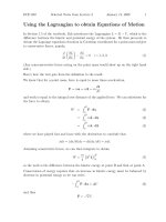
FRF of "
The first mode is
present as an antiresonance

:8;<+1=>132!5!&17.18

The two modes
are clearly present

!'!&

:8;<+1=>132!5!&17.1"

FRF of h

632!5!&617.18

!'!&(

!
!!'(
!&
!&'(
!"

!"'(
!9

!

"

#
$
)*+,-+./012345

%

&!


Working with the FRF
•! If the force is non-sinusoidal, F0=F0(!).
•! The system’s response to such a force is
obtained as q0(!)=H(!)-1F(!).
•! If F(!)=1 then the inverse Fourier
Transform of q0(!) is the system’s impulse
response.
•! The impulse response can also be used to
perform stability analysis.
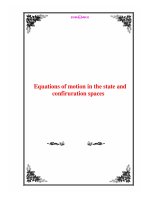
Introduction to Aeroelasticity


Impulse response of
pitch-plunge airfoil

!)

!#

9:&),;/<('=;>:!?#

'(&!

&'(
2-3450.*6.03780.*,8*9

1,234/-(5-/267/-(+7(8

#
"
!
!"
!#
!$

!

"

#

$

%

&!

&"

&#

&$

&%

:;"(-<0=*)>
)*&!

&
!'(
!
!!'(
!&
!&'(

!

"

#

$

%

*+,-(./0
!#

&"

&#

&$

&%

&!

&"

&#

&$

&%

!#

'(&!

)*&!

2-3450.*6.03780.*,8*!

1,234/-(5-/267/-(+7(!

"

&!
+,-.*/01

!

"

!

!"
!"

!

"

#

$

%

&!
*+,-(./0

V=15m/s

Introduction to Aeroelasticity

&"

&#

&$

&%

!

"

#

$

%
+,-.*/01

V=25m/s


Damped sinusoidal motion
•! The previous discussion shows that:

–! Theodorsen aerodynamics are only valid for
sinusoidal motion
–! Yet Theodorsen aerodynamics can be used to

calculate damped impulse responses

•! Stability analysis is slow and and can be less
accurate when performed on impulse
responses
•! We need a method for calculating the
damping at all airspeeds directly from the
equations of motion
Introduction to Aeroelasticity


The p-k Method
•! The p-k method is the most popular
technique for obtaining aeroelastic
solutions
•! It was started in the 80s and since then
has become the industrial standard
•! Virtually all aircraft flying today have
been designed using the p-k method
Introduction to Aeroelasticity


Basics

•! The p-k method uses the structural
equations of motion in the standard
form
•! Coupled with Theodorsen aerodynamic
forces of the form

With k=!b/U
Introduction to Aeroelasticity


Basics (2)
•! Remember that this is only correct if the
response is sinusoidal, since the
Theodorsen lift is equal to

•! The p-k method mixes h(t), which is a
general function, with h0expj!t.
Introduction to Aeroelasticity


Basics (3)
•! Therefore, the equations contain terms
that depend on frequency
•! The basis of the p-k method is to define
•! Then, the equations of motion become
1
$ 2
&
2
p M s + K s " #U Q( p) q = 0
%
'
2

•! Where q=[h "]T.
Introduction to Aeroelasticity

Using p!
•! Using the p notation, the Q(p) matrix
becomes:
2
(
p
2$ p&
"2#cC ( k ) " 2#b
*
%U'
U
*
*
Q( p) = *
2
c& 2$ p&
p
$
2
*2#ec C ( k ) + 2# x f " b
%
2' % U '
U
*
*)

p
$3

& p
$ p&
"2#cC ( k ) " 2#b
" 2#cC ( k ) c " x f
" 2#b 2
%4
'U
%U'
U
p
$3
&
2#ec 2C ( k ) " 2 c " x f #b 2 +
%4
'
U

•! i.e. it is a polynomial function of p (or p/U).
Introduction to Aeroelasticity

2

+
2
2
24
p
3
p
b

p
c
$
&
$
& $ &
$ & " 2#b 2 x f "
"#
2#ec 2C ( k ) c " x f
%4
'U
%
2' % U '
4 % U ' -,
2


The p-method
•! The p-method consists of solving this
eigenvalue problem for p.
1
$ 2
&
p M s + K s " #U 2Q( p) q = 0
%
'
2

•! It’s a nonlinear eigenvalue problem but
polynomial so it can be solved.

•! The p values will generally be complex.
•! There is no guarantee that the real parts of
the p values will have the correct value
Introduction to Aeroelasticity


The p-k method
•! The p-k method is more sophisticated than
the p-method in that it performs frequency
matching
•! The equations solved are
1
$ 2
&
p M s + K s " #U 2Q( jk ) q = 0
%
'
2

(2)

•! Since it is known that the aerodynamic
matrix is only a function of frequency (not
of damping)
•! Again, k=!b/U
Introduction to Aeroelasticity


Application to 2-dof model
•! The p-k equations for the 2-dof model

are:
#
%
%
%# m
% %$ S
%
%
$

S & 2 #Kk
(p +%
I" '
$0

,
)4+C ( k ) jk + 2+k 2
.
.
0& 1
2.
( ) *U .
c& 2
#
K" ' 2
k
(
)
4
+

ecC
k
jk
)
2
+
x
)
.
$ f 2'
.
.-

/&
#3
&
)2+cC ( k ) ) 2+bjk ) 4+C ( k ) c ) x f jk + 2+b 2 k 2 1(
$4
'
1(
#3
&
2
1( 2 h 5 = 0
2+ec C ( k ) ) 2 c ) x f +bjk +
6
$4
'
1( 3
4" 7

1(
2
b 2 2 1(
c& 2
#3
&
#
k ++ k
4+ecC ( k ) c ) x f jk + 2+ x f )
$4
'
$
2'
4 10'

•! Notice that the Q matrix depends only
on k, not on flight condition
Introduction to Aeroelasticity


The p-k solution
•! The solution of these equations is iterative.
•! We guess a value for the frequency ! (and
hence k) and then we calculate p from the
resulting eigenvalue problem.
•! The norm of p should be equal to !.
•! If it is not, we change the value of ! until the
scheme converges
•! This is called frequency matching
Introduction to Aeroelasticity

Frequency matching

Introduction to Aeroelasticity


p-k method characteristics
•! Converges very quickly to the correct
eigenvalue
•! Suitable for large computational
problems
•! Calculates sub-critical damping ratios
•! Flutter speeds are very similar to the kmethod results
Introduction to Aeroelasticity


Results

Introduction to Aeroelasticity


Roger’s Approximation
•! Another way to transform the p-k equations to
the time domain is using Roger’s
Approximation.
•! The frequency-dependent part of equations
(2), Q(jk), is approximated as:
2

nl

Q( jk ) = A 0 + A1 jk + A 2 ( jk ) + # A 2+n
n =1

jk
jk + " n

•! Where nl is the number of aerodynamic lags
and "n are aerodynamic lag coefficients.
Introduction to Aeroelasticity


Roger’s EOMs

•! The equations of motion of the complete
aeroelastic system then become:
$ "M "1C "M "1K "M "1A 3 ! "M "1A n l +2 '
& I
)
0
0
!
0
&
)
I
"V# 1 /bI !
0
q˙ = & 0

)q
& "
)
"
"
#
"
&&
))
I
0
! "V# n l /bI (
% 0

•! Where

1
1
1
1
M = M s " #b 2A 2 , C = Cs " #UbA1, K = K s " #U 2A 0 , A j = " #U 2A j
2
2
2
2

•! Usually:

n l = 4, " n = #1.7kmax
Introduction to Aeroelasticity

n

(nl + 1)

2

, kmax = maximum k of interest


Practical Aeroelasticity
•! For an aircraft, the matrix Q(jk) is obtained using a
panel method-based aerodynamic model.
•! The modelling is usually performed by means of
commercial packages, such as MSC.Nastran or ZAero.
•! For a chosen set of k values, e.g. k1, k2, !, km, the
corresponding Q matrices are returned.
•! The Q matrices are then used in conjunction with
the p-k method to obtain the flutter solution or
time-domain responses.
•! The values of Q at intermediate k values are
obtained by interpolation.
Introduction to Aeroelasticity


BAH Example
•! Bisplinghoff, Ashley and Halfman wing

•! FEM with 12 nodes and 72 dof
Introduction to Aeroelasticity

First 5 modes of BAH wing

Introduction to Aeroelasticity


GTA Example
•! Here is a very simple aeroelastic model for
a Generic Transport Aircraft

Finite element model: Bar elements
with 678 degrees of freedom
Introduction to Aeroelasticity

Aerodynamic model: 2500 doublet
lattice panels