Cpu Scheduling: Proportional Share
Bạn đang xem bản rút gọn của tài liệu. Xem và tải ngay bản đầy đủ của tài liệu tại đây (93.17 KB, 10 trang )
9
Scheduling: Proportional Share
In this chapter, we’ll examine a different type of scheduler known as a
proportional-share scheduler, also sometimes referred to as a fair-share
scheduler. Proportional-share is based around a simple concept: instead
of optimizing for turnaround or response time, a scheduler might instead
try to guarantee that each job obtain a certain percentage of CPU time.
An excellent modern example of proportional-share scheduling is found
in research by Waldspurger and Weihl [WW94], and is known as lottery
scheduling; however, the idea is certainly much older [KL88]. The basic
idea is quite simple: every so often, hold a lottery to determine which process should get to run next; processes that should run more often should
be given more chances to win the lottery. Easy, no? Now, onto the details!
But not before our crux:
C RUX : H OW T O S HARE T HE CPU P ROPORTIONALLY
How can we design a scheduler to share the CPU in a proportional
manner? What are the key mechanisms for doing so? How effective are
they?
9.1 Basic Concept: Tickets Represent Your Share
Underlying lottery scheduling is one very basic concept: tickets, which
are used to represent the share of a resource that a process (or user or
whatever) should receive. The percent of tickets that a process has represents its share of the system resource in question.
Let’s look at an example. Imagine two processes, A and B, and further
that A has 75 tickets while B has only 25. Thus, what we would like is for
A to receive 75% of the CPU and B the remaining 25%.
Lottery scheduling achieves this probabilistically (but not deterministically) by holding a lottery every so often (say, every time slice). Holding
a lottery is straightforward: the scheduler must know how many total
tickets there are (in our example, there are 100). The scheduler then picks
1
2
S CHEDULING : P ROPORTIONAL S HARE
T IP : U SE R ANDOMNESS
One of the most beautiful aspects of lottery scheduling is its use of randomness. When you have to make a decision, using such a randomized
approach is often a robust and simple way of doing so.
Random approaches has at least three advantages over more traditional
decisions. First, random often avoids strange corner-case behaviors that a
more traditional algorithm may have trouble handling. For example, consider the LRU replacement policy (studied in more detail in a future chapter on virtual memory); while often a good replacement algorithm, LRU
performs pessimally for some cyclic-sequential workloads. Random, on
the other hand, has no such worst case.
Second, random also is lightweight, requiring little state to track alternatives. In a traditional fair-share scheduling algorithm, tracking how
much CPU each process has received requires per-process accounting,
which must be updated after running each process. Doing so randomly
necessitates only the most minimal of per-process state (e.g., the number
of tickets each has).
Finally, random can be quite fast. As long as generating a random number is quick, making the decision is also, and thus random can be used
in a number of places where speed is required. Of course, the faster the
need, the more random tends towards pseudo-random.
a winning ticket, which is a number from 0 to 991 . Assuming A holds
tickets 0 through 74 and B 75 through 99, the winning ticket simply determines whether A or B runs. The scheduler then loads the state of that
winning process and runs it.
Here is an example output of a lottery scheduler’s winning tickets:
63 85 70 39 76 17 29 41 36 39 10 99 68 83 63 62 43
0 49 49
Here is the resulting schedule:
A
A
B
A
A
B
A
A
A
A
A
A
B
A
A
A
A
A
A
B
As you can see from the example, the use of randomness in lottery
scheduling leads to a probabilistic correctness in meeting the desired proportion, but no guarantee. In our example above, B only gets to run 4 out
of 20 time slices (20%), instead of the desired 25% allocation. However,
the longer these two jobs compete, the more likely they are to achieve the
desired percentages.
1
Computer Scientists always start counting at 0. It is so odd to non-computer-types that
famous people have felt obliged to write about why we do it this way [D82].
O PERATING
S YSTEMS
[V ERSION 0.90]
WWW. OSTEP. ORG
S CHEDULING : P ROPORTIONAL S HARE
3
T IP : U SE T ICKETS T O R EPRESENT S HARES
One of the most powerful (and basic) mechanisms in the design of lottery
(and stride) scheduling is that of the ticket. The ticket is used to represent
a process’s share of the CPU in these examples, but can be applied much
more broadly. For example, in more recent work on virtual memory management for hypervisors, Waldspurger shows how tickets can be used to
represent a guest operating system’s share of memory [W02]. Thus, if you
are ever in need of a mechanism to represent a proportion of ownership,
this concept just might be ... (wait for it) ... the ticket.
9.2 Ticket Mechanisms
Lottery scheduling also provides a number of mechanisms to manipulate tickets in different and sometimes useful ways. One way is with
the concept of ticket currency. Currency allows a user with a set of tickets to allocate tickets among their own jobs in whatever currency they
would like; the system then automatically converts said currency into the
correct global value.
For example, assume users A and B have each been given 100 tickets.
User A is running two jobs, A1 and A2, and gives them each 500 tickets
(out of 1000 total) in User A’s own currency. User B is running only 1 job
and gives it 10 tickets (out of 10 total). The system will convert A1’s and
A2’s allocation from 500 each in A’s currency to 50 each in the global currency; similarly, B1’s 10 tickets will be converted to 100 tickets. The lottery
will then be held over the global ticket currency (200 total) to determine
which job runs.
User A -> 500 (A’s currency) to A1 -> 50 (global currency)
-> 500 (A’s currency) to A2 -> 50 (global currency)
User B -> 10 (B’s currency) to B1 -> 100 (global currency)
Another useful mechanism is ticket transfer. With transfers, a process
can temporarily hand off its tickets to another process. This ability is
especially useful in a client/server setting, where a client process sends
a message to a server asking it to do some work on the client’s behalf.
To speed up the work, the client can pass the tickets to the server and
thus try to maximize the performance of the server while the server is
handling the client’s request. When finished, the server then transfers the
tickets back to the client and all is as before.
Finally, ticket inflation can sometimes be a useful technique. With
inflation, a process can temporarily raise or lower the number of tickets
it owns. Of course, in a competitive scenario with processes that do not
trust one another, this makes little sense; one greedy process could give
itself a vast number of tickets and take over the machine. Rather, inflation
can be applied in an environment where a group of processes trust one
another; in such a case, if any one process knows it needs more CPU time,
it can boost its ticket value as a way to reflect that need to the system, all
without communicating with any other processes.
c 2014, A RPACI -D USSEAU
T HREE
E ASY
P IECES
4
S CHEDULING : P ROPORTIONAL S HARE
1
2
// counter: used to track if we’ve found the winner yet
int counter = 0;
3
4
5
6
// winner: use some call to a random number generator to
//
get a value, between 0 and the total # of tickets
int winner = getrandom(0, totaltickets);
7
8
9
// current: use this to walk through the list of jobs
node_t *current = head;
10
11
12
13
14
15
16
17
18
// loop until the sum of ticket values is > the winner
while (current) {
counter = counter + current->tickets;
if (counter > winner)
break; // found the winner
current = current->next;
}
// ’current’ is the winner: schedule it...
Figure 9.1: Lottery Scheduling Decision Code
9.3
Implementation
Probably the most amazing thing about lottery scheduling is the simplicity of its implementation. All you need is a good random number
generator to pick the winning ticket, a data structure to track the processes of the system (e.g., a list), and the total number of tickets.
Let’s assume we keep the processes in a list. Here is an example comprised of three processes, A, B, and C, each with some number of tickets.
head
Job:A
Tix:100
Job:B
Tix:50
Job:C
Tix:250
NULL
To make a scheduling decision, we first have to pick a random number
(the winner) from the total number of tickets (400)2 Let’s say we pick the
number 300. Then, we simply traverse the list, with a simple counter
used to help us find the winner (Figure 9.1).
The code walks the list of processes, adding each ticket value to counter
until the value exceeds winner. Once that is the case, the current list element is the winner. With our example of the winning ticket being 300,
the following takes place. First, counter is incremented to 100 to account for A’s tickets; because 100 is less than 300, the loop continues.
Then counter would be updated to 150 (B’s tickets), still less than 300
and thus again we continue. Finally, counter is updated to 400 (clearly
greater than 300), and thus we break out of the loop with current pointing at C (the winner).
To make this process most efficient, it might generally be best to organize the list in sorted order, from the highest number of tickets to the
2
¨
Surprisingly, as pointed out by Bjorn
Lindberg, this can be challenging to do
correctly; for more details, see />how-to-generate-a-random-number-from-within-a-range.
O PERATING
S YSTEMS
[V ERSION 0.90]
WWW. OSTEP. ORG
S CHEDULING : P ROPORTIONAL S HARE
5
1.0
Unfairness (Average)
0.8
0.6
0.4
0.2
0.0
1
10
100
Job Length
1000
Figure 9.2: Lottery Fairness Study
lowest. The ordering does not affect the correctness of the algorithm;
however, it does ensure in general that the fewest number of list iterations are taken, especially if there are a few processes that possess most
of the tickets.
9.4 An Example
To make the dynamics of lottery scheduling more understandable, we
now perform a brief study of the completion time of two jobs competing
against one another, each with the same number of tickets (100) and same
run time (R, which we will vary).
In this scenario, we’d like for each job to finish at roughly the same
time, but due to the randomness of lottery scheduling, sometimes one
job finishes before the other. To quantify this difference, we define a
simple unfairness metric, U which is simply the time the first job completes divided by the time that the second job completes. For example,
if R = 10, and the first job finishes at time 10 (and the second job at 20),
= 0.5. When both jobs finish at nearly the same time, U will be
U = 10
20
quite close to 1. In this scenario, that is our goal: a perfectly fair scheduler
would achieve U = 1.
Figure 9.2 plots the average unfairness as the length of the two jobs
(R) is varied from 1 to 1000 over thirty trials (results are generated via the
simulator provided at the end of the chapter). As you can see from the
graph, when the job length is not very long, average unfairness can be
quite severe. Only as the jobs run for a significant number of time slices
does the lottery scheduler approach the desired outcome.
c 2014, A RPACI -D USSEAU
T HREE
E ASY
P IECES
6
S CHEDULING : P ROPORTIONAL S HARE
9.5
How To Assign Tickets?
One problem we have not addressed with lottery scheduling is: how
to assign tickets to jobs? This problem is a tough one, because of course
how the system behaves is strongly dependent on how tickets are allocated. One approach is to assume that the users know best; in such a
case, each user is handed some number of tickets, and a user can allocate
tickets to any jobs they run as desired. However, this solution is a nonsolution: it really doesn’t tell you what to do. Thus, given a set of jobs,
the “ticket-assignment problem” remains open.
9.6
Why Not Deterministic?
You might also be wondering: why use randomness at all? As we saw
above, while randomness gets us a simple (and approximately correct)
scheduler, it occasionally will not deliver the exact right proportions, especially over short time scales. For this reason, Waldspurger invented
stride scheduling, a deterministic fair-share scheduler [W95].
Stride scheduling is also straightforward. Each job in the system has
a stride, which is inverse in proportion to the number of tickets it has. In
our example above, with jobs A, B, and C, with 100, 50, and 250 tickets,
respectively, we can compute the stride of each by dividing some large
number by the number of tickets each process has been assigned. For
example, if we divide 10,000 by each of those ticket values, we obtain
the following stride values for A, B, and C: 100, 200, and 40. We call
this value the stride of each process; every time a process runs, we will
increment a counter for it (called its pass value) by its stride to track its
global progress.
The scheduler then uses the stride and pass to determine which process should run next. The basic idea is simple: at any given time, pick
the process to run that has the lowest pass value so far; when you run
a process, increment its pass counter by its stride. A pseudocode implementation is provided by Waldspurger [W95]:
current = remove_min(queue);
schedule(current);
current->pass += current->stride;
insert(queue, current);
//
//
//
//
pick client with minimum pass
use resource for quantum
compute next pass using stride
put back into the queue
In our example, we start with three processes (A, B, and C), with stride
values of 100, 200, and 40, and all with pass values initially at 0. Thus, at
first, any of the processes might run, as their pass values are equally low.
Assume we pick A (arbitrarily; any of the processes with equal low pass
values can be chosen). A runs; when finished with the time slice, we
update its pass value to 100. Then we run B, whose pass value is then
set to 200. Finally, we run C, whose pass value is incremented to 40. At
this point, the algorithm will pick the lowest pass value, which is C’s, and
run it, updating its pass to 80 (C’s stride is 40, as you recall). Then C will
O PERATING
S YSTEMS
[V ERSION 0.90]
WWW. OSTEP. ORG
S CHEDULING : P ROPORTIONAL S HARE
Pass(A)
(stride=100)
0
100
100
100
100
100
200
200
200
Pass(B)
(stride=200)
0
0
200
200
200
200
200
200
200
Pass(C)
(stride=40)
0
0
0
40
80
120
120
160
200
7
Who Runs?
A
B
C
C
C
A
C
C
...
Figure 9.3: Stride Scheduling: A Trace
run again (still the lowest pass value), raising its pass to 120. A will run
now, updating its pass to 200 (now equal to B’s). Then C will run twice
more, updating its pass to 160 then 200. At this point, all pass values are
equal again, and the process will repeat, ad infinitum. Figure 9.3 traces
the behavior of the scheduler over time.
As we can see from the figure, C ran five times, A twice, and B just
once, exactly in proportion to their ticket values of 250, 100, and 50. Lottery scheduling achieves the proportions probabilistically over time; stride
scheduling gets them exactly right at the end of each scheduling cycle.
So you might be wondering: given the precision of stride scheduling,
why use lottery scheduling at all? Well, lottery scheduling has one nice
property that stride scheduling does not: no global state. Imagine a new
job enters in the middle of our stride scheduling example above; what
should its pass value be? Should it be set to 0? If so, it will monopolize
the CPU. With lottery scheduling, there is no global state per process;
we simply add a new process with whatever tickets it has, update the
single global variable to track how many total tickets we have, and go
from there. In this way, lottery makes it much easier to incorporate new
processes in a sensible manner.
9.7 Summary
We have introduced the concept of proportional-share scheduling and
briefly discussed two implementations: lottery and stride scheduling.
Lottery uses randomness in a clever way to achieve proportional share;
stride does so deterministically. Although both are conceptually interesting, they have not achieved wide-spread adoption as CPU schedulers
for a variety of reasons. One is that such approaches do not particularly
mesh well with I/O [AC97]; another is that they leave open the hard problem of ticket assignment, i.e., how do you know how many tickets your
browser should be allocated? General-purpose schedulers (such as the
MLFQ we discussed previously, and other similar Linux schedulers) do
so more gracefully and thus are more widely deployed.
c 2014, A RPACI -D USSEAU
T HREE
E ASY
P IECES
8
S CHEDULING : P ROPORTIONAL S HARE
As a result, proportional-share schedulers are more useful in domains
where some of these problems (such as assignment of shares) are relatively easy to solve. For example, in a virtualized data center, where you
might like to assign one-quarter of your CPU cycles to the Windows VM
and the rest to your base Linux installation, proportional sharing can be
simple and effective. See Waldspurger [W02] for further details on how
such a scheme is used to proportionally share memory in VMWare’s ESX
Server.
O PERATING
S YSTEMS
[V ERSION 0.90]
WWW. OSTEP. ORG
S CHEDULING : P ROPORTIONAL S HARE
9
References
[AC97] “Extending Proportional-Share Scheduling to a Network of Workstations”
Andrea C. Arpaci-Dusseau and David E. Culler
PDPTA’97, June 1997
A paper by one of the authors on how to extend proportional-share scheduling to work better in a
clustered environment.
[D82] “Why Numbering Should Start At Zero”
Edsger Dijkstra, August 1982
/>A short note from E. Dijkstra, one of the pioneers of computer science. We’ll be hearing much more
on this guy in the section on Concurrency. In the meanwhile, enjoy this note, which includes this
motivating quote: “One of my colleagues — not a computing scientist — accused a number of younger
computing scientists of ’pedantry’ because they started numbering at zero.” The note explains why
doing so is logical.
[KL88] “A Fair Share Scheduler”
J. Kay and P. Lauder
CACM, Volume 31 Issue 1, January 1988
An early reference to a fair-share scheduler.
[WW94] “Lottery Scheduling: Flexible Proportional-Share Resource Management”
Carl A. Waldspurger and William E. Weihl
OSDI ’94, November 1994
The landmark paper on lottery scheduling that got the systems community re-energized about scheduling, fair sharing, and the power of simple randomized algorithms.
[W95] “Lottery and Stride Scheduling: Flexible
Proportional-Share Resource Management”
Carl A. Waldspurger
Ph.D. Thesis, MIT, 1995
The award-winning thesis of Waldspurger’s that outlines lottery and stride scheduling. If you’re thinking of writing a Ph.D. dissertation at some point, you should always have a good example around, to
give you something to strive for: this is such a good one.
[W02] “Memory Resource Management in VMware ESX Server”
Carl A. Waldspurger
OSDI ’02, Boston, Massachusetts
The paper to read about memory management in VMMs (a.k.a., hypervisors). In addition to being
relatively easy to read, the paper contains numerous cool ideas about this new type of VMM-level
memory management.
c 2014, A RPACI -D USSEAU
T HREE
E ASY
P IECES
10
S CHEDULING : P ROPORTIONAL S HARE
Homework
This program, lottery.py, allows you to see how a lottery scheduler
works. See the README for details.
Questions
1. Compute the solutions for simulations with 3 jobs and random seeds
of 1, 2, and 3.
2. Now run with two specific jobs: each of length 10, but one (job 0)
with just 1 ticket and the other (job 1) with 100 (e.g., -l 10:1,10:100).
What happens when the number of tickets is so imbalanced? Will
job 0 ever run before job 1 completes? How often? In general, what
does such a ticket imbalance do to the behavior of lottery scheduling?
3. When running with two jobs of length 100 and equal ticket allocations of 100 (-l 100:100,100:100), how unfair is the scheduler?
Run with some different random seeds to determine the (probabilistic) answer; let unfairness be determined by how much earlier one
job finishes than the other.
4. How does your answer to the previous question change as the quantum size (-q) gets larger?
5. Can you make a version of the graph that is found in the chapter?
What else would be worth exploring? How would the graph look
with a stride scheduler?
O PERATING
S YSTEMS
[V ERSION 0.90]
WWW. OSTEP. ORG