estimation techniques tutorial
Bạn đang xem bản rút gọn của tài liệu. Xem và tải ngay bản đầy đủ của tài liệu tại đây (1.5 MB, 59 trang )
Estimation Techniques
About the Tutorial
Estimation techniques are of utmost importance in software development life cycle, where
the time required to complete a particular task is estimated before a project begins.
Estimation is the process of finding an estimate, or approximation, which is a value that
can be used for some purpose even if input data may be incomplete, uncertain,
or unstable. This tutorial discusses various estimation techniques such as estimation using
Function Points, Use-Case Points, Wideband Delphi technique, PERT, Analogy, et
Audience
If you are an aspiring project manager or project leader, then this tutorial is definitely for
you. It will take you through all the important estimation techniques.
Prerequisites
Before proceeding with this tutorial, you should have a basic understanding of the Software
Development Life Cycle (SDLC). In addition, you should have a basic understanding of
software programming using any programming language.
Disclaimer & Copyright
Copyright 2015 by Tutorials Point (I) Pvt. Ltd.
All the content and graphics published in this e-book are the property of Tutorials Point (I)
Pvt. Ltd. The user of this e-book is prohibited to reuse, retain, copy, distribute or republish
any contents or a part of contents of this e-book in any manner without written consent
of the publisher.
We strive to update the contents of our website and tutorials as timely and as precisely as
possible, however, the contents may contain inaccuracies or errors. Tutorials Point (I) Pvt.
Ltd. provides no guarantee regarding the accuracy, timeliness or completeness of our
website or its contents including this tutorial. If you discover any errors on our website or
in this tutorial, please notify us at
i
Estimation Techniques
Table of Contents
About the Tutorial .................................................................................................................................... i
Audience .................................................................................................................................................. i
Prerequisites ............................................................................................................................................ i
Disclaimer & Copyright............................................................................................................................. i
Table of Contents .................................................................................................................................... ii
1.
ESTIMATION – OVERVIEW ................................................................................................... 1
Observations on Estimation .................................................................................................................... 1
General Project Estimation Approach ..................................................................................................... 2
Estimation Accuracy ................................................................................................................................ 3
Estimation Issues .................................................................................................................................... 3
Estimation Guidelines ............................................................................................................................. 4
2.
FUNCTION POINTS............................................................................................................... 6
ISO Standards .......................................................................................................................................... 6
Object Management Group Specification for Automated Function Point ................................................ 6
History of Function Point Analysis ........................................................................................................... 6
Elementary Process (EP) .......................................................................................................................... 7
Functions ................................................................................................................................................ 7
Definition of RETs, DETs, FTRs ................................................................................................................. 9
3.
FP COUNTING PROCESS..................................................................................................... 10
Step 1: Determine the Type of Count .................................................................................................... 10
Step 2: Determine the Boundary of the Count ...................................................................................... 11
Step 3: Identify Each Elementary Process Required by the User ............................................................ 11
Step 4: Determine the Unique Elementary Processes ............................................................................ 11
Step 5: Measure Data Functions ............................................................................................................ 11
Step 6: Measure Transactional Functions .............................................................................................. 13
ii
Estimation Techniques
Step 7: Calculate Functional Size (Unadjusted Function Point Count) .................................................... 18
Benefits of Function Points ................................................................................................................... 21
FP Repositories ..................................................................................................................................... 22
4.
USE-CASE POINTS .............................................................................................................. 23
Use-Case Points – Definition ................................................................................................................. 23
History of Use-Case Points .................................................................................................................... 23
Use-Case Points Counting Process ......................................................................................................... 23
Advantages and Disadvantages of Use-Case Points ............................................................................... 29
5.
WIDEBAND DELPHI TECHNIQUE ........................................................................................ 30
Wideband Delphi Technique – Steps ..................................................................................................... 30
Advantages and Disadvantages of Wideband Delphi Technique ........................................................... 33
6.
THREE-POINT ESTIMATION ................................................................................................ 35
Standard Deviation ............................................................................................................................... 35
Convert the Project Estimates to Confidence Levels .............................................................................. 36
7.
PROJECT EVALUATION & REVIEW TECHNIQUE .................................................................. 37
Standard Deviation ............................................................................................................................... 37
PERT Estimation Steps ........................................................................................................................... 38
Convert the Project Estimates to Confidence Levels .............................................................................. 38
Differences between Three-Point Estimation and PERT ........................................................................ 39
8.
ANALOGOUS ESTIMATION................................................................................................. 40
Analogous Estimation – Definition ........................................................................................................ 40
Analogous Estimation Requirements .................................................................................................... 40
Analogous Estimation Steps .................................................................................................................. 41
Advantages of Analogous Estimation .................................................................................................... 41
iii
Estimation Techniques
9.
WORK BREAKDOWN STRUCTURE ...................................................................................... 42
Representation of WBS ......................................................................................................................... 42
Types of WBS ........................................................................................................................................ 44
Estimate Size ......................................................................................................................................... 44
Estimate Effort ...................................................................................................................................... 44
Scheduling ............................................................................................................................................. 45
Critical Path Method ............................................................................................................................. 45
Task Dependency Relationships ............................................................................................................ 45
Gantt Chart ........................................................................................................................................... 46
Milestones ............................................................................................................................................ 47
Advantages of Estimation using WBS .................................................................................................... 47
10. PLANNING POKER .............................................................................................................. 48
Planning Poker Estimation .................................................................................................................... 48
Planning Poker Estimation Technique ................................................................................................... 48
Benefits of Planning Poker Estimation .................................................................................................. 49
11. TESTING ESTIMATION TECHNIQUES .................................................................................. 50
Percentage of Development Effort Method .......................................................................................... 50
Testing Estimation Techniques .............................................................................................................. 51
iv
1. Estimation – Overview
Estimation Techniques
Estimation is the process of finding an estimate, or approximation, which is a value that
can be used for some purpose even if input data may be incomplete, uncertain,
or unstable.
Estimation determines how much money, effort, resources, and time it will take to build a
specific system or product. Estimation is based on:
Past Data/Past Experience
Available Documents/Knowledge
Assumptions
Identified Risks
The four basic steps in Software Project Estimation are:
Estimate the size of the development product.
Estimate the effort in person-months or person-hours.
Estimate the schedule in calendar months.
Estimate the project cost in agreed currency.
Observations on Estimation
Estimation need not be a one-time task in a project. It can take place during:
o Acquiring a Project.
o
Planning the Project.
o
Execution of the Project as the need arises.
Project scope must be understood before the estimation process begins. It will be
helpful to have historical Project Data.
Project metrics can provide a historical perspective and valuable input for
generation of quantitative estimates.
Planning requires technical managers and the software team to make an initial
commitment as it leads to responsibility and accountability.
Past experience can aid greatly.
Use at least two estimation techniques to arrive at the estimates and reconcile the
resulting values. Refer Decomposition Techniques in the next section to learn about
reconciling estimates.
Plans should be iterative and allow adjustments as time passes and more details
are known.
1
Estimation Techniques
General Project Estimation Approach
The Project Estimation Approach that is widely used is Decomposition Technique.
Decomposition techniques take a divide and conquer approach. Size, Effort and Cost
estimation are performed in a stepwise manner by breaking down a Project into major
Functions or related Software Engineering Activities.
Step 1: Understand the scope of the software to be built.
Step 2: Generate an estimate of the software size.
o
Start with the statement of scope.
o
Decompose the software into functions that can each be estimated individually.
o
Calculate the size of each function.
o
Derive effort and cost estimates by applying the size values to your baseline
productivity metrics.
o
Combine function estimates to produce an overall estimate for the entire project.
Step 3: Generate an estimate of the effort and cost. You can arrive at the effort and cost
estimates by breaking down a project into related software engineering activities.
o
Identify the sequence of activities that need to be performed for the project to be
completed.
o
Divide activities into tasks that can be measured.
o
Estimate the effort (in person hours/days) required to complete each task.
o
Combine effort estimates of tasks of activity to produce an estimate for the
activity.
o
Obtain cost units (i.e., cost/unit effort) for each activity from the database.
o
Compute the total effort and cost for each activity.
o
Combine effort and cost estimates for each activity to produce an overall effort
and cost estimate for the entire project.
Step 4: Reconcile estimates: Compare the resulting values from Step 3 to those obtained
from Step 2. If both sets of estimates agree, then your numbers are highly reliable.
Otherwise, if widely divergent estimates occur conduct further investigation concerning
whether:
o
The scope of the project is not adequately understood or has been misinterpreted.
o
The function and/or activity breakdown is not accurate.
o
Historical data used for the estimation techniques is inappropriate for the
application, or obsolete, or has been misapplied.
Step 5: Determine the cause of divergence and then reconcile the estimates.
2
Estimation Techniques
Estimation Accuracy
Accuracy is an indication of how close something is to reality. Whenever you generate an
estimate, everyone wants to know how close the numbers are to reality. You will want
every estimate to be as accurate as possible, given the data you have at the time you
generate it. And of course you don’t want to present an estimate in a way that inspires a
false sense of confidence in the numbers.
Important factors that affect the accuracy of estimates are:
The accuracy of all the estimate’s input data.
The accuracy of any estimate calculation.
How closely the historical data or industry data used to calibrate the model matches
the project you are estimating.
The predictability of your organization’s software development process.
The stability of both the product requirements and the environment that supports
the software engineering effort.
Whether or not the actual project was carefully planned, monitored and controlled,
and no major surprises occurred that caused unexpected delays.
Following are some guidelines for achieving reliable estimates:
Base estimates on similar projects that have already been completed.
Use relatively simple decomposition techniques to generate project cost and effort
estimates.
Use one or more empirical estimation models for software cost and effort
estimation.
Refer to the section on Estimation Guidelines in this chapter.
To ensure accuracy, you are always advised to estimate using at least two techniques
and compare the results.
Estimation Issues
Often, project managers resort to estimating schedules skipping to estimate size. This may
be because of the timelines set by the top management or the marketing team. However,
whatever the reason, if this is done, then at a later stage it would be difficult to estimate
the schedules to accommodate the scope changes.
While estimating, certain assumptions may be made. It is important to note all these
assumptions in the estimation sheet, as some still do not document assumptions in
estimation sheets.
Even good estimates have inherent assumptions, risks, and uncertainty, and yet they are
often treated as though they are accurate.
3
Estimation Techniques
The best way of expressing estimates is as a range of possible outcomes by saying, for
example, that the project will take 5 to 7 months instead of stating it will be complete on
a particular date or it will be complete in a fixed no. of months. Beware of committing to
a range that is too narrow as that is equivalent to committing to a definite date.
You could also include uncertainty as an accompanying probability value. For
example, there is a 90% probability that the project will complete on or before a
definite date.
Organizations do not collect accurate project data. Since the accuracy of the
estimates depend on the historical data, it would be an issue.
For any project, there is a shortest possible schedule that will allow you to include
the required functionality and produce quality output. If there is a schedule
constraint by management and/or client, you could negotiate on the scope and
functionality to be delivered.
Agree with the client on handling scope creeps to avoid schedule overruns.
Failure in accommodating contingency in the final estimate causes issues. For e.g.,
meetings, organizational events.
Resource utilization should be considered as less than 80%. This is because the
resources would be productive only for 80% of their time. If you assign resources
at more than 80% utilization, there is bound to be slippages.
Estimation Guidelines
One should keep the following guidelines in mind while estimating a project:
During estimation, ask other people's experiences. Also, put your own experiences
at task.
Assume resources will be productive for only 80 percent of their time. Hence, during
estimation take the resource utilization as less than 80%.
Resources working on multiple projects take longer to complete tasks because of
the time lost switching between them.
Include management time in any estimate.
Always build in contingency for problem solving, meetings and other unexpected
events.
Allow enough time to do a proper project estimate. Rushed estimates are
inaccurate, high-risk estimates. For large development projects, the estimation
step should really be regarded as a mini project.
Where possible, use documented data from your organization’s similar past
projects. It will result in the most accurate estimate. If your organization has not
kept historical data, now is a good time to start collecting it.
4
Estimation Techniques
Use developer-based estimates, as the estimates prepared by people other than
those who will do the work will be less accurate.
Use several different people to estimate and use several different estimation
techniques.
Reconcile the estimates. Observe the convergence or spread among the estimates.
Convergence means that you have got a good estimate. Wideband-Delphi
technique can be used to gather and discuss estimates using a group of people,
the intention being to produce an accurate, unbiased estimate.
Re-estimate the project several times throughout its life cycle.
5
2. Function Points
Estimation Techniques
A Function Point (FP) is a unit of measurement to express the amount of business
functionality, an information system (as a product) provides to a user. FPs measure
software size. They are widely accepted as an industry standard for functional sizing.
For sizing software based on FP, several recognized standards and/or public specifications
have come into existence. As of 2013, these are:
ISO Standards
COSMIC: ISO/IEC 19761:2011 Software
measurement method.
engineering.
A
functional
size
FiSMA: ISO/IEC 29881:2008 Information technology - Software and systems
engineering - FiSMA 1.1 functional size measurement method.
IFPUG: ISO/IEC 20926:2009 Software and systems engineering - Software
measurement - IFPUG functional size measurement method.
Mark-II: ISO/IEC 20968:2002 Software engineering - Ml II Function Point
Analysis - Counting Practices Manual.
NESMA: ISO/IEC 24570:2005 Software engineering - NESMA function size
measurement method version 2.1 - Definitions and counting guidelines for the
application of Function Point Analysis.
Object Management Group Specification for Automated Function Point
Object Management Group (OMG), an open membership and not-for-profit computer
industry standards consortium, has adopted the Automated Function Point (AFP)
specification led by the Consortium for IT Software Quality. It provides a standard for
automating FP counting according to the guidelines of the International Function Point
User Group (IFPUG).
Function Point Analysis (FPA) technique quantifies the functions contained within
software in terms that are meaningful to the software users. FPs consider the number of
functions being developed based on the requirements specification.
Function Points (FP) Counting is governed by a standard set of rules, processes and
guidelines as defined by the International Function Point Users Group (IFPUG). These are
published in Counting Practices Manual (CPM).
History of Function Point Analysis
The concept of Function Points was introduced by Alan Albrecht of IBM in 1979. In 1984,
Albrecht refined the method. The first Function Point Guidelines were published in 1984.
The International Function Point Users Group (IFPUG) is a US-based worldwide
organization of Function Point Analysis metric software users. The International
6
Estimation Techniques
Function Point Users Group (IFPUG) is a non-profit, member-governed organization
founded in 1986. IFPUG owns Function Point Analysis (FPA) as defined in ISO standard
20296:2009 which specifies the definitions, rules and steps for applying the IFPUG's
functional size measurement (FSM) method. IFPUG maintains the Function Point Counting
Practices Manual (CPM). CPM 2.0 was released in 1987, and since then there have been
several iterations. CPM Release 4.3 was in 2010.
The CPM Release 4.3.1 with incorporated ISO editorial revisions was in 2010. The ISO
Standard (IFPUG FSM) - Functional Size Measurement that is a part of CPM 4.3.1 is a
technique for measuring software in terms of the functionality it delivers. The CPM is an
internationally approved standard under ISO/IEC 14143-1 Information Technology –
Software Measurement.
Elementary Process (EP)
Elementary Process is the smallest unit of functional user requirement that:
Is meaningful to the user.
Constitutes a complete transaction.
Is self-contained and leaves the business of the application being counted in a
consistent state.
Functions
There are two types of functions:
Data Functions
Transaction Functions
Data Functions
There are two types of data functions:
Internal Logical Files
External Interface Files
Data Functions are made up of internal and external resources that affect the system.
Internal Logical Files
Internal Logical File (ILF) is a user identifiable group of logically related data or control
information that resides entirely within the application boundary. The primary intent of an
ILF is to hold data maintained through one or more elementary processes of the application
being counted. An ILF has the inherent meaning that it is internally maintained, it has
some logical structure and it is stored in a file. (Refer Figure 1)
External Interface Files
External Interface File (EIF) is a user identifiable group of logically related data or control
information that is used by the application for reference purposes only. The data resides
entirely outside the application boundary and is maintained in an ILF by another
7
Estimation Techniques
application. An EIF has the inherent meaning that it is externally maintained, an interface
has to be developed to get the data from the file. (Refer Figure 1)
Figure 1: Application Boundary, Data Functions, Transaction Functions
Transaction Functions
There are three types of transaction functions.
External Inputs
External Outputs
External Inquiries
Transaction functions are made up of the processes that are exchanged between the
user, the external applications and the application being measured.
External Inputs
External Input (EI) is a transaction function in which Data goes “into” the application from
outside the boundary to inside. This data is coming external to the application.
Data may come from a data input screen or another application.
An EI is how an application gets information.
Data can be either control information or business information.
Data may be used to maintain one or more Internal Logical Files.
If the data is control information, it does not have to update an Internal Logical
File. (Refer Figure 1)
8
Estimation Techniques
External Outputs
External Output (EO) is a transaction function in which data comes “out” of the system.
Additionally, an EO may update an ILF. The data creates reports or output files sent to
other applications. (Refer Figure 1)
External Inquiries
External Inquiry (EQ) is a transaction function with both input and output components
that result in data retrieval. (Refer Figure 1)
Definition of RETs, DETs, FTRs
Record Element Type
A Record Element Type (RET) is the largest user identifiable subgroup of elements within
an ILF or an EIF. It is best to look at logical groupings of data to help identify them.
Data Element Type
Data Element Type (DET) is the data subgroup within an FTR. They are unique and user
identifiable.
File Type Referenced
File Type Referenced (FTR) is the largest user identifiable subgroup within the EI, EO, or
EQ that is referenced to.
The transaction functions EI, EO, EQ are measured by counting FTRs and DETs that they
contain following counting rules. Likewise, data functions ILF and EIF are measured by
counting DETs and RETs that they contain following counting rules. The measures of
transaction functions and data functions are used in FP counting which results in the
functional size or function points.
9
3. FP Counting Process
Estimation Techniques
FP Counting Process involves the following steps:
Step 1: Determine the type of count.
Step 2: Determine the boundary of the count.
Step 3: Identify each Elementary Process (EP) required by the user.
Step 4: Determine the unique EPs.
Step 5: Measure data functions.
Step 6: Measure transactional functions.
Step 7: Calculate functional size (unadjusted function point count).
Step 8: Determine Value Adjustment Factor (VAF).
Step 9: Calculate adjusted function point count.
Note: General System Characteristics (GSCs) are made optional in CPM 4.3.1 and moved
to Appendix. Hence, Step 8 and Step 9 can be skipped.
Step 1: Determine the Type of Count
There are three types of function point counts:
Development Function Point Count
Application Function Point Count
Enhancement Function Point Count
Development Function Point Count
Function points can be counted at all phases of a development project from requirement
to implementation stage. This type of count is associated with new development work and
may include the prototypes, which may have been required as temporary solution, which
supports the conversion effort. This type of count is called a baseline function point count.
Application Function Point Count
Application counts are calculated as the function points delivered, and exclude any
conversion effort (prototypes or temporary solutions) and existing functionality that may
have existed.
Enhancement Function Point Count
When changes are made to software after production, they are considered as
enhancements. To size such enhancement projects, the Function Point Count gets Added,
Changed or Deleted in the Application.
10
Estimation Techniques
Step 2: Determine the Boundary of the Count
The boundary indicates the border between the application being measured and the
external applications or the user domain. (Refer Figure 1)
To determine the boundary, understand:
The purpose of the function point count
Scope of the application being measured
How and which applications maintain what data
The business areas that support the applications
Step 3: Identify Each Elementary Process Required by the User
Compose and/or decompose the functional user requirements into the smallest unit of
activity, which satisfies all of the following criteria:
Is meaningful to the user.
Constitutes a complete transaction.
Is self-contained.
Leaves the business of the application being counted in a consistent state.
For example, the Functional User Requirement – “Maintain Employee information” can be
decomposed into smaller activities such as add employee, change employee, delete
employee, and inquire about employee.
Each unit of activity thus identified is an Elementary Process (EP).
Step 4: Determine the Unique Elementary Processes
Comparing two EPs already identified, count them as one EP (same EP) if they:
Require the same set of DETs.
Require the same set of FTRs.
Require the same set of processing logic to complete the EP.
Do not split an EP with multiple forms of processing logic into multiple Eps.
For e.g., if you have identified ‘Add Employee’ as an EP, it should not be divided into two
EPs to account for the fact that an employee may or may not have dependents. The EP is
still ‘Add Employee’, and there is variation in the processing logic and DETs to account for
dependents.
Step 5: Measure Data Functions
Classify each data function as either an ILF or an EIF.
A data function shall be classified as an:
Internal Logical File (ILF), if it is maintained by the application being measured.
11
Estimation Techniques
External Interface File (EIF) if it is referenced, but not maintained by the application
being measured.
ILFs and EIFs can contain business data, control data and rules based data. For example,
telephone switching is made of all three types - business data, rule data and control data.
Business data is the actual call. Rule data is how the call should be routed through the
network, and control data is how the switches communicate with each other.
Consider the following documentation for counting ILFs and EIFs:
Objectives and constraints for the proposed system.
Documentation regarding the current system, if such a system exists.
Documentation of the users’ perceived objectives, problems and needs.
Data models.
Step 5.1: Count the DETs for Each Data Function
Apply the following rules to count DETs for ILF/EIF:
Count a DET for each unique user identifiable, non-repeated field maintained in or
retrieved from the ILF or EIF through the execution of an EP.
Count only those DETs being used by the application that is measured when two or
more applications maintain and/or reference the same data function.
Count a DET for each attribute required by the user to establish a relationship with
another ILF or EIF.
Review related attributes to determine if they are grouped and counted as a single
DET or whether they are counted as multiple DETs. Grouping will depend on how
the EPs use the attributes within the application.
Step 5.2: Count the RETs for Each Data Function
Apply the following rules to count RETs for ILF/EIF:
Count one RET for each data function.
Count
DETs.
o
o
o
one additional RET for each of the following additional logical sub-groups of
Associative entity with non-key attributes.
Sub-type (other than the first sub-type).
Attributive entity, in a relationship other than mandatory 1:1.
12
Estimation Techniques
Step 5.3: Determine the Functional Complexity for Each Data Function
Data Element Types (DETs)
RETS
1-19
20-50
>50
1
L
L
A
2 to 5
L
A
H
>5
A
H
H
Table 1: ILF/EIF Complexity Matrix
Functional Complexity: L=Low; A=Average; H=High
Step 5.4: Measure the Functional Size for Each Data Function
Functional
Complexity
FP Count
for ILF
FP Count
for EIF
Low
7
5
Average
10
7
High
15
10
Table 2: ILF/EIF FP Counts
Step 6: Measure Transactional Functions
To measure transactional functions following are the necessary steps:
Step 6.1: Classify each Transactional Function
Transactional functions should be classified as an External Input, External Output or an
External Inquiry.
External Input
External Input (EI) is an Elementary Process that processes data or control information
that comes from outside the boundary. The prima ry intent of an EI is to maintain one or
more ILFs and/or to alter the behavior of the system.
All of the following rules must be applied:
The data or control information is received from outside the application boundary.
At least one ILF is maintained if the data entering the boundary is not control
information that alters the behavior of the system.
For the identified EP, one of the three statements must apply:
o
Processing logic is unique from processing logic performed by other EIs for
the application.
o
The set of data elements identified is different from the sets identified for
other EIs in the application.
13
Estimation Techniques
o
ILFs or EIFs referenced are different from the files referenced by the other
EIs in the application.
External Output
External Output (EO) is an Elementary Process that sends data or control information
outside the application’s boundary. EO includes additional processing beyond that of an
external inquiry.
The primary intent of an EO is to present information to a user through processing logic
other than or in addition to the retrieval of data or control information.
The processing logic must:
Contain at least one mathematical formula or calculation.
Create derived data.
Maintain one or more ILFs.
Alter the behavior of the system.
All of the following rules must be applied:
Sends data or control information external to the application’s boundary.
For the identified EP, one of the three statements must apply:
o
Processing logic is unique from the processing logic performed by other EOs
for the application.
o
The set of data elements identified are different from other EOs in the
application.
o
ILFs or EIFs referenced are different from files referenced by other EOs in the
application.
Additionally, one of the following rules must apply:
The processing logic contains at least one mathematical formula or calculation.
The processing logic maintains at least one ILF.
The processing logic alters the behavior of the system.
External Inquiry
External Inquiry (EQ) is an Elementary Process that sends data or control information
outside the boundary. The primary intent of an EQ is to present information to the user
through the retrieval of data or control information.
The processing logic contains no mathematical formula or calculations, and creates no
derived data. No ILF is maintained during the processing, nor is the behavior of the system
altered.
All of the following rules must be applied:
Sends data or control information external to the application’s boundary.
14
Estimation Techniques
For the identified EP, one of the three statements must apply:
o
Processing logic is unique from the processing logic performed by other EQs
for the application.
o
The set of data elements identified are different from other EQs in the
application.
o
The ILFs or EIFs referenced are different from the files referenced by other
EQs in the application.
Additionally, all of the following rules must apply:
The processing logic retrieves data or control information from an ILF or EIF.
The processing logic does not contain mathematical formula or calculation.
The processing logic does not alter the behavior of the system.
The processing logic does not maintain an ILF.
Step 6.2: Count the DETs for Each Transactional Function
Apply the following Rules to count DETs for EIs:
Review everything that crosses (enters and/or exits) the boundary.
Count one DET for each unique user identifiable, non-repeated attribute that
crosses (enters and/or exits) the boundary during the processing of the
transactional function.
Count only one DET per transactional function for the ability to send an application
response message, even if there are multiple messages.
Count only one DET per transactional function for the ability to initiate action(s)
even if there are multiple means to do so.
Do not count the following items as DETs:
o
Attributes generated within the boundary by a transactional function and
saved to an ILF without exiting the boundary.
o
Literals such as report titles, screen or panel identifiers, column headings and
attribute titles.
o
Application generated stamps such as date and time attributes.
o
Paging variables, page numbers and positioning information, for e.g., ‘Rows
37 to 54 of 211’.
o
Navigation aids such as the ability to navigate within a list using “previous”,
“next”, “first”, “last” and their graphical equivalents.
15
Estimation Techniques
Apply the following rules to count DETs for EOs/EQs:
Review everything that crosses (enters and/or exits) the boundary.
Count one DET for each unique user identifiable, non-repeated attribute that
crosses (enters and/or exits) the boundary during the processing of the
transactional function.
Count only one DET per transactional function for the ability to send an application
response message, even if there are multiple messages.
Count only one DET per transactional function for the ability to initiate action(s)
even if there are multiple means to do so.
Do not count the following items as DETs:
o
Attributes generated within the boundary without crossing the boundary.
o
Literals such as report titles, screen or panel identifiers, column headings and
attribute titles.
o
Application generated stamps such as date and time attributes.
o
Paging variables, page numbers and positioning information, for e.g., ‘Rows
37 to 54 of 211’.
o
Navigation aids such as the ability to navigate within a list using “previous”,
“next”, “first”, “last” and their graphical equivalents.
Step 6.3: Count the FTRs for Each Transactional Function
Apply the following rules to count FTRs for EIs:
Count a FTR for each ILF maintained.
Count a FTR for each ILF or EIF read during the processing of the EI.
Count only one FTR for each ILF that is both maintained and read.
Apply the following rule to count FTRs for EO/EQs:
Count a FTR for each ILF or EIF read during the processing of EP.
Additionally, apply the following rules to count FTRs for EOs:
Count a FTR for each ILF maintained during the processing of EP.
Count only one FTR for each ILF that is both maintained and read by EP.
16
Estimation Techniques
Step 6.4: Determine the Functional Complexity for Each Transactional
Function
Data Element Types (DETs)
FTRs
1-4
5-15
>=16
0-1
L
L
A
2
L
A
H
>=3
A
H
H
Table 3: EI Complexity Matrix
Functional Complexity: L=Low; A=Average; H=High
Determine the functional complexity for each EO/EQ, with an exception that EQ must have
a minimum of 1 FTR:
EQ must
have a
minimum
of 1 FTR
Data Element Types (DETs)
1-4
5-15
>=16
0-1
L
L
A
2
L
A
H
>=3
A
H
H
FTRs
Table 4: EO/EQ Functional Complexity Matrix
Functional Complexity: L=Low; A=Average; H=High
Step 6.5: Measure the Functional Size for Each Transactional Function
Measure the functional size for each EI from its functional complexity.
Complexity
FP Count
Low
3
Average
4
High
6
Table 5: EI FP Counts
17
Estimation Techniques
Measure the functional size for each EO/EQ from its functional complexity.
Complexity
FP Count
for EO
FP Count
for EQ
Low
4
3
Average
5
4
High
6
6
Table 6: EO/EQ FP Counts
Step 7: Calculate Functional Size (Unadjusted Function Point Count)
To calculate the functional size, one should follow the steps given below:
Step 7.1
Recollect what you have found in Step 1. Determine the type of count.
Step 7.2
Calculate the functional size or function point count based on the type.
For development function point count, go to Step 7.3.
For application function point count, go to Step 7.4.
For enhancement function point count, go to Step 7.5.
Step 7.3
Development Function Point Count consists of two components of functionality:
Application functionality included in the user requirements for the project.
Conversion functionality included in the user requirements for the project.
Conversion functionality consists of functions provided only at installation to
convert data and/or provide other user-specified conversion requirements, such as
special conversion reports. For e.g. an existing application may be replaced with a
new system.
DFP = ADD + CFP
Where,
DFP = Development Function Point Count
ADD = Size of functions delivered to the user by the development project
CFP = Size of the conversion functionality
ADD = FP Count (ILFs) + FP Count (EIFs) + FP Count (EIs) + FP Count (EOs) + FP Count (EQs)
CFP = FP Count (ILFs) + FP Count (EIFs) + FP Count (EIs) + FP Count (EOs) + FP Count (EQs)
18
Estimation Techniques
Step 7.4
Calculate the Application Function Point Count
AFP = ADD
Where,
AFP = Application Function Point Count
ADD = Size of functions delivered to the user by the development project
(excluding the size of any conversion functionality), or the functionality that exists
whenever the application is counted.
ADD = FP Count (ILFs) + FP Count (EIFs) + FP Count (EIs) + FP Count (EOs) + FP Count (EQs)
Step 7.5
Enhancement Function Point Count considers the following four components of
functionality:
Functionality that is added to the application.
Functionality that is modified in the Application.
Conversion functionality.
Functionality that is deleted from the application.
EFP =ADD + CHGA + CFP + DEL
Where,
EFP = Enhancement Function Point Count
ADD = Size of functions being added by the enhancement project
CHGA = Size of functions being changed by the enhancement project
CFP = Size of the conversion functionality
DEL = Size of functions being deleted by the enhancement project
ADD = FP Count (ILFs) + FP Count (EIFs) + FP Count (EIs) + FP Count (EOs) + FP Count (EQs)
CHGA = FP Count (ILFs) + FP Count (EIFs) + FP Count (EIs) + FP Count (EOs) + FP Count (EQs)
CFP = FP Count (ILFs) + FP Count (EIFs) + FP Count (EIs) + FP Count (EOs) + FP Count (EQs)
DEL = FP Count (ILFs) + FP Count (EIFs) + FP COUNT (EIs) + FP Count (EOs) + FP Count (EQs)
Step 8: Determine the Value Adjustment Factor
GSCs are made optional in CPM 4.3.1 and moved to Appendix. Hence, Step 8 and Step 9
can be skipped.
19
Estimation Techniques
The Value Adjustment Factor (VAF) is based on 14 GSCs that rate the general functionality
of the application being counted. GSCs are user business constraints independent of
technology. Each characteristic has associated descriptions to determine the degree of
influence.
General System
Characteristic
Brief Description
Data Communications
How many communication facilities are there to aid in the
transfer or exchange of information with the application
or system?
Distributed Data
Processing
How are distributed data and processing functions
handled?
Performance
Did the user require response time or throughput?
Heavily Used Configuration
How heavily used is the current hardware platform where
the application will be executed?
Transaction Rate
How frequently are transactions executed daily, weekly,
monthly, etc.?
On-Line Data Entry
What percentage of the information is entered online?
End-user Efficiency
Was the application designed for end-user efficiency?
Online Update
How many ILFs are updated by online transaction?
Complex Processing
Does the application have extensive logical or
mathematical processing?
Reusability
Was the application developed to meet one or many user’s
needs?
Installation Ease
How difficult is conversion and installation?
Operational Ease
How effective and/or automated are start-up, back-up,
and recovery procedures?
Multiple Sites
Was the application specifically designed, developed, and
supported to be installed at multiple sites for multiple
organizations?
Facilitate Change
Was the application specifically designed, developed, and
supported to facilitate change?
Table 7: General System Characteristics (GSCs)
20