PARALLELIZATION OF ALGORITHMS IN GRAPH NETWORK
Bạn đang xem bản rút gọn của tài liệu. Xem và tải ngay bản đầy đủ của tài liệu tại đây (407.83 KB, 26 trang )
MINISTRY OF EDUCATION AND TRAINING
DA NANG UNIVERSITY
----- -----
NGUYEN DINH LAU
PARALLELIZATION OF ALGORITHMS
IN GRAPH NETWORK
SPECIALIZATION: COMPUTER SCIENCE
CODE: 62.48.01.01
PHD. THESIS IN BRIEF
DA NANG - 2016
This thesis has been finished at:
Danang University of Technology, Da Nang University
Supervisor:
1. Ass. Prof. DrSc. TRAN QUOC CHIEN
2. Ass. Prof. PhD. LE MANH THANH
Examiner 1: Ass. Prof. PhD. Doan Van Ban
Examiner 2: Ass. Prof. PhD. Nguyen Mau Han
Examiner 3: PhD. Huynh Huu Hung
The PhD. Thesis was defended at the Thesis Assessment
Committee at Da Nang University Level at Room No:
Da Nang University
At 8.30 am January 24th 2016
The thesis is available at:
1. The National Library.
2. The Information Resources Center, University of Danang.
1
PREFACE
1. Significance of the study
When building sequential algorithms for problems on the graphic
network, the algorithms themselves are not only very complex but the
complexity of the algorithms also is very big. Thus, sequential
algorithms must be parralled to share work and reduce computation
time.
For above reasons, it is crucial to build
parallelization of
algorithms in extended graph to find the shortest path and to find
maximum flow. Therefore, a study of “Parallelization of algorithms in
graph network” is essential to deal with many real problems with huge
input data in our daily life
2. Objects and Scope of the study
Objects of the study
- Investigating and discovering parallel processing theory,
parallel processing models.
- Investigating graphic theory, mainly focus on parallel
algorithms to find the shortest and to find the maximum flow.
Scope of the study
- Suggesting parallel algorithms to find the shortest path for the
two vertexes in extended graph.
- Suggesting parallel algorithms finding the maximum flow by Preflowpush methods, Suggesting parallel algorithms to find the maximum
flow by Postflow-pull methods, Suggesting parallel algorithms to find
concurent max flow with bounded cost in extended graph.
3. New findings of the study
- Suggesting arallel algorithms to find the shortest path in
extended network. So far, parallel algorithms have been built in
2
traditional graphs. In this thesis, the first new parallel algorithms are
especially built for real transport network, prove complexity.
- Suggesting parallel algorithms to find maximum flow by
Preflow-push methods. A new feature here is the sequential and parallel
algorithms are carefully demonstrated, the algorithms also consider
several unexpected cases to occur in the process. Experimental section
is made clear. Besides, the program is built on a cluster computer
system. Finally, the results are skillfully compared and fully
commented.
- Suggesting parallel algorithms to find the maximum flow by
combined flow push and pull methods. New feature here is that the new
algorithm built has not been announced, the theorems are proven, the
experimental examples were built specifically.
- Suggesting new parallel algorithms finding the concurent max
flow with bounded cost in extended graph. New feature here is that the
new algorithm buil thas not been announced, the theorems are proven.
4. Results of the study
-Suggesting a new parallel algorithms based on the actual
requirements, proving soundness, the complexity of the algorithms.
Concurently, thesis also does parallelization for existing algorithms,
then indicate the advantages of the new ones over previous algorithms.
- Developing experimental programs on various parallel systems,
then offering specific data to evaluate and compare the results of new
parallel algorithms with sequential algorithms or with the other previous
parallel algorithms.
5. Table of contents
Besides preface, conclusion, references, the thesis has four
chapters:
3
Chapter 1. Parallel processing.
Chapter 2. Sequential and parallel algorithms in tradition graph
network
Chapter 3. parallel algorithms to find the shortest path and
maximum flow in extended graph network.
4
CHAPTER 1
PARALLEL PROCESSING
1.1. Introduction of parallel processing
1.2. Architectures of parallel computers
1.3. Paralell algorithm
1.4. Conclusion
To deal with the problems effectively in our computer, The key
here is we have to build parallel algorithms. The common way we do is
to convert the sequential algorithms into parallel algorithms, or convert
parallel algorithms into other suitable parallel algorithms which are
totally equal to the original algorithms.
To evaluate the effectiveness of parallel algorithms, we usually
based on the complexity of the algorithms. The complexity of parallel
algorithms depends not only on the volume of input data but also on the
the architecture of the computer as well as the number of proceesors in
the system.
5
CHAPTER 2. SEQUENTIAL AND PARALLEL
ALGORITHMS IN TRADITION GRAPH NETWORK
2.1. Network and flow
2.2. The problem of maximum flow
2.3. Pre-fow push algorithm to find maximum flow
2.3.1. Sequential algorithm
2.3.1.1. Introduction
2.3.1.2. Some basic concept
Residual network Gf:
For flow f on G = (V, E, c), where a is source vertex, z is sink
vertex, c is capacity. Residual network, denoted Gf is defined as the
network with a set of vertices V and a set of edge Ef with the capacity
as follows:
- for any edge (u, v) E, if f(u, v)> 0, then (v, u) Ef with capacity
is cf(v, u)=f(u, v)
- for any edge (u, v) E, if c(u, v) -f(u, v) > 0, then (u, v) Ef with
capacity is cf(u,v) = c(u, v) - f(u,v)
Pre-flow:
For network G = (V, E, c). Preflow is a set of
flows on the edges f = {fi, j | (i, j) E} So that
(i) 0 fi, j ci, j(i, j) E
(ii) for any vertex k is not a source or sink, inflow is not smaller
than outflow, that is
f i, k
(i , k )E
Height function:
fk, j
( k , j )E
6
Height function of the pre-flow in the network G = (V, E, c) is a set
of non-negative vertex weights h(0), ..., h(|V| 1) such that h(z) = 0 for z
and h(u) ≤ h(v) + 1 for every edge (u, v) in the residual network for the
flow. An eligible edge is an edge (u, v) in the residual network with
h(u) = h(v) + 1.
2.3.1.3. Preflow-push algorithm
- Input: G = (V, E, c), a is source vertex, z is sink , capacity
c= {ci, j | (i, j) E}
- Output: Maximum Flow:
f = {fi, j | (i, j) E}
Step 1:
Initialized: building the initial pre-flow in the edges leaving the
source to the sink vertices, which is filled to capacity, the other flows
are 0. Choose height function h(v) which is the length of the shortest
path from v to vertex z.
Push all unbalanced vertices into the queue Q.
Step 2:
Condition to terminate: If Q=, then preflow f becomes max
flow, end. If Q, go to Step 3.
Step 3:
How to perform unbalanced vertex: get unbalanced vertex u from
the queue.
Browsing the priority edges (u, v) Ef. Pull along the edge (u, v)
a flow with value min{delta, cf(u, v)}, where deltais the excess of the
vertex u.
- If vertex v is the new unbalanced vertex, then push this vertex v
into queue Q.
-
If vertex u is still unbalanced, then increase the height of the
vertex u as follows:
7
h(u): =1 +min{h(v) |(u, v) Ef }
and push u into the queue Q.
Back to step2.
2.3.1.4. For example
2.3.2. Parallel algorithm
2.3.2.1. Introduction
2.3.2.2. The idea of the parallel algorithm
2.3.2.3. Building the parallel algorithm
- Input: Graph G(V, E, c) with source a, sink z, the capacity:
c= {ci, j | (i, j) E}
m processors (P0, P1,…, Pm-1), where P0 is the main processor
- Output: Maximum flow:
f = {fi, j | (i, j) E}
Step 1: The main processor P0 performs
(1.1). initialize: e, h, f, cf, Q: set of unbalanced vertices (excluding the
vertices a and z) are the vertices with positive excess.
(1.2). divide set of vertices V into sub-processors:
Let Pi be the ith sub-processor (i = 1, 2, ..., m-1).
Pi will receive the set of vertices Vi so that:
{
(
)
Step 2: sub-processors Pi receive Vi (i=1,…,m-1)
Step 3: The main processor checks if Q= then end, f becomes
maximum flow, else to step 4
Step 4: Main processor send e, h, f, c, cf to the sub-processors.
Step 5: m-1 sub-processors (P1, P2, …,Pm-1) implement
8
(5.1) Receive e, h, f, c, cf and the set of vertices from the main processor
(5.2) Handling unbalanced vertice v (push and replace label) as in Step
3 of the sequential algorithm. Get unbalanced vertexs v (e(v)>0) from Q
and vVi (i= 1, 2, ..., m-1). Browsing the priority edges (u, v) Gf.
Push along edge (u, v) a flow with valuel min{delta, cf(u, v)}, where
delta is the excess of vertex u.
If it does not exist the priority edge fromv, then increased the
hight of the vertex u as follows:
h(u)= 1 + min{h(v) | (u, v) Ef}
(5.3) Send e, h, f, c, cf, to the main processor
Step 6: The main processor implements
(6.1) Receive e, h, f, c, cf from step 5.3
(6.2) This step is distinctive from the sequential algorithms to
synchronize our data, after receiving the data in (6.1), the main
processor checks if all the edges u, v E that have h(u)> h(v)+1, the
main processor will relabel for vertices u, v as follows:
f(u, v)= f(u, v)+min{delta, cf(u, v);
e(u)= e(u)–cf(u, v);
e(v)= e(v)+cf(u, v)
Put the new unbalanced vertex into set Q.
(6.3) If u V e(u)=0, eliminate u from active set Q.
Back to step 3.
2.3.2.4. For example
2.3.2.5. Analyse complexity
2.3.2.6. Execute results
Speedup (Ts/Tp)
9
Number of processors
Fugire 2.12. Chartper forms the speedup of graph having
7000 nodes and 5000 nodes
2.3.2.7. Conclusion
2.4. Combined flow push and pull algorithm
2.4.1. Postflow-pull algorithm
2.4.1.1. Introduction
2.4.1.2. Some basic concept
Postflow
For network G = (V, E, c). Postflow is a set of flows on the edges
f = {fi, j | (i, j) E}
So that
(i) 0 fi, j ci, j(i, j) E
(ii) for any vertex k is not a source or sink, outflow is not smaller
than inflow, that is:
f i, k f k , j
(i , k )E
( k , j )E
10
Depth function of the flow in the network G = (V, E, c) is a set of nonnegative vertex weights d(0), ..., d(|V| 1) such that d(a) = 0 for a and
d(u) + 1 d(v) for every edge (u, v) in the residual network for the
flow. An eligible edge is an edge (u, v) in the residual network with
d(u)+1=d(v).
2.4.1.3. Postflow-pull algorithm
- Input:
G = (V, E, c), a is source vertex, z is sink , capacity:
c= {ci, j | (i, j) E}
- Output:
Maximum Flow
f = {fi, j | (i, j) E
Step 1:
Initialized: building the initial postflow in the edges leaving the
source to the sink vertices, which is filled to capacity, the other flows
are 0. Choose depth function d(v) which is the length of the shortest
path from source a to vertex v.
Push all unbalanced vertices into the queue Q.
Step 2:
Condition to terminate: If Q=, then postflow f becomes max
flow, end. If Q, go to Step 3.
Step 3:
How to perform unbalanced vertex: get unbalanced vertex v from
the queue.
Browsing the priority edges (u, v) Gf. Pull along the edge (u, v)
a flow with value min{delta, cf(u, v)}, where delta(<0) is the excess of
the vertex v. If vertex u is the new unbalanced vertex, then push this
vertex u into queue Q.
11
If vertex v is still unbalanced, then increase the depth of the
vertex v as follows:
d(v): =1 +min{d(u) |(u, v) Ef }
then push v into the queue Q.
Back to Step 2.
2.4.1.4. For example
2.4.2. Combined flow push and pull algorithm
This is new algorithm to find maximum flow. Combined
algorithm preflow-push and method postflow-pull to build the
algorithm combined flow push and pull as follows:
2.4.2.1. Combined flow push and pull algorithm
This is a particular algorithm in combined flow push and pull
method. Here the unbalanced positive vertices are push into the queue
Q+ and the unbalanced negative vertices are push into the queue Q-.
With each vertex from the queue Q+, we will push the flow in the
priority edge until the vertex becomes either balanced or does not have
any priority edge. If it does not exist priority edge but there are
unbalanced vertices, then we increase the height and push it into the
queue Q+.
With each vertex from the queue Q-, we will pull the flow in the
priority edge until the vertex becomes either balanced or does not have
any priority edge. If it does not exist priority edge but there are
unbalanced vertices, then we increase the depth and push it into the
queue Q-.
2.4.2.2. For example
2.4.3. Parallel aglorithm combined flow push and pull
2.4.3.1. Itroduction
Preflow-push algorithm and postflow-pull algorithm combined
the flow push and pull algorithm all of them have complexity O(|V|2|E|).
12
To reduce the computer time of this combined the flow push and pull
algorithm, we build this algorithm on multiple processors
2.4.3.2. The idea of the parallel algorithm
Parallel algorithms using 3 processors P0, P1, P3. In 3 processors,
there is a main processor (P0) to manage data, divide data into 2 subprocessors (P1, P2). Sub-processors P1 push flow from Q+.
Sub-processors P2 pull flow from Q-. The processors finish when all P1,
P2 to qual null.
2.4.3.3. Building the parallel algorithm
Input: Graph G (V, E, c) with source a, sink z, the capacity
c= {ci, j | (i, j) E}
Three processors (P0, P1, P2), where P0 is the main processor
Output: Maximum flow
f = {fi, j | (i, j) E
Step 1: The main processor P0 performs
- initialize: h, d, e, f, c, Q+, QStep 2: The main processor checks
- Receive datas from the sub-processors
- Checks if Q+, Q- is null and P1, P2 all of them finish, then f is
maximum flow, Stop.
Else go to Step 3.
Step 3: The main processor checks
- Get node u from Q+ and y from Q- Send h, e, f, u, Q+ to P1. Send d, e, f, node y, Q- to P2
- The main processor checks: If any the priority edges(u, v) Ef
and any the priority edges(x, y)Ef so that u=x or y=v then go to
Step 5.
Else go to Step 4
13
Step 4: Sub-processors P1 and P2 parallel performs
- Two sub-processorsReceive datas from the main processor
- Processor P1 performs
Preflow-push
Send Q+, h, e, f, cf to the main processor
- Processor P2 performs
postflow-pull
Send Q-, d, e, f to the main processor.
Back to Step 2
Step 5: Sub-processors P1 and P2 sequential performs
- Processor P1 performs
Receive datas from P0 send to in Step 3
Preflow-push
- Processor P2 performs:
Receive datas from P0 send to in Step 3 and receive data from P1
send to in Step 5
postflow-pull
Send Q-, d, e, f to the main processor.
Back to Step 2.
2.4.3.4. For example
2.4.3.4. Conclusion
2.5. Chapter Conclusion
In chapter two, we have carefully presented preflow-push
algorithm inherited from previous studies and have suggested
Combined flow push and pull to find maximum flow. After that we
optimize Parallel aglorithm preflow-push and propose Parallel
aglorithm combined flow push and pull to find maximum flow. The
parallel
algorithms
are
thoroughly
presented.
The
theorems,
propositions and consequences related to the algorithms are clearly
14
demonstrated. The parallel algorithms analyse computation time. In
particular, the main content of this chapter is published in three
Information Technology journals and listed in [1], [3], [4] in the
portfolio of the writer.
15
CHAPTER 3. PARALLEL ALGORITHMS TO FIND THE
SHORTEST PATH AND MAXIMUM FLOW IN EXTENDED
GRAPH NETWORK
3.1. Extended graph
Given extended graph G(V, E) with a set of vertices V and a set of
edges E, where edges can be directed or undirected. Each edge E is
weighted wE(e). With each vertex vV, Ev is the set of edges of vertex v.
Each vertex vV and each edge(e, e') Ev xEv, e≠e' is weighted
wV(v, e, e').
A set (V, E, wE, wV) is called extended graph.
3.2. Extended traffic network
Given a graph network G(V, E) with a set of vertices V and a set
of edges E, where edges can be directed or undirected. The functions in
network as follows:
For cE edge capacity function: ER*, then cE(e) is edge capacity
e E
For cV vertices capacity function: VR*, then cV(u) is vertices
capacity u V.
For bE edge cost function: ER*, then bE(e): cost must be return
to transfer an unit transport on edge e
With each vV, Set Ev is a set of edge of vertice v.
For bV vertices cost function: VEvEvR*, bV(u,e,e‟): cost must
be paid to transfer commodity from edge e to vertice u to edge e‟.
A set (V, E, cE, cV, bE, bV) is called extended traffic network.
3.3. Algorithm finding the shortest path in extended graph
3.3.1. Sequential Algorithm
3.3.1.1. Introduction
3.3.1.2. Building the sequential algorithm
16
- Input: Extended graph G(V, E, wE, wV), vertex s, tV
-Output: l(v) is the length of the shortest path from s to t and the
shortest path (if l(v) <+∞)
- Steps.
The algorithm uses the following symbols:
S is a set of vertices that found the shortest path starting from s.
T=V-S; l(v) is the length of the shortest path from s to v;
VE={(v, e)|vV\{s}& eEV} {(s, )} is the set of vertices and
edges;
SE is a set of vertex-edge excluded from VE;
TE=VE-SE;
L(v, e) is the vertex-edge pair label (v, e) VE
P(v, e) is the vertex- front edge (v, e) VE
Step 1. (Initialized) Let S = ; T=V;
Let VE={(v, e)|vV\{s}& eEV} {(s, )} SE= ; TE=VE;
Set L(v, e)=∞, (v, e) VE, L(s, ):=0.
Set P(v, e)= (v, e) VE
Step 2. Calculate m = min{L((v, e))| (v, e) TE}.
If m=+∞. Not path. The end.
Else, if m<+∞, choose (vmin, emin) TE so that L(vmin, emin)=m,
Set TE=TE-{(vmin, emin)}, SE=SE {(vmin, emin)}, go to step 3.
Step 3. If vmin S , then set le(vmin)=emin, S=S vmin , l(vmin)=L(vmin ,
emin), T=T-{vmin}.
-if t vmin then go to step 5, else go to step 4.
Step 4. For any (v, e) TE adjacent (post-adjacent) (vmin, emin),
Set L’(v, e)=L(vmin, emin)+wE(vmin, v)+ wV(vmin, emin, e), if vmin s
and L‟(v, e)=L(s, )+ wE(vmin, v) if vmin = s.
IF L(v, e)>L‟(v, e), then set L(v, e)=L‟(v, e) and P(v, e)= (vmin,
emin) Back to step 2.
17
Step 5. (Finding the shortest path)
Set l(t)=L(t, le(t)) is the length of the shortest path from s to t.
From t tracing back the front vertex-edge, we receive the shortest
path as following: let (v1, e1)=P(t, le(t)), (v2, e2)=P(v1, e1), …, (vk,
ek) =P(vk-1, ek-1), (s, )= P(vk, ek).
The shortest path is:
s vk vk 1 ... v1 t .
The end.
Theorem 3.1. The algorithm finding the shortest path from s vertex to t
vertices in the extended graph is true.
Theorem3.2. Let G be the extended graph having n vertices. The
algorithm has complexity O(n3).
3.3.2. Parallel algorithm
3.3.2.1. Introduction
3.3.2.2. The idea of the parallel algorithm
We build parallel algorithms on k processors (P0, P1,…,Pk-1). In k
processors, there is a main processor (P0) to manage data, divide data
into k-1 sub-processors (P1,…,Pk-1) Sub-processors receive the data
from the main processor and find minximun L(v, e) on their vertices and
send it to main processor. The main processor will find L(vmin, emin)
=min(Li(v, e)), i=0,…,k-1) which sub-processors sent.
Next, The main processor will send (vmin, emin ) to sub-processors
to calculate.
3.3.2.3. Building the parallel algorithm
3.3.2.4. Execute results
Speedup (Ts/Tp)
18
Number of processors
Fugire 3.4. The speedup of graph having 7000 nodes and 5000 nodes
3.3.2.5. Conclusion
3.4. Algorithm finding concurent max flow with bounded cost
3.4.1. Sequential algorithm
3.4.1.1. Introduction
3.4.1.2. Problem finding concurent max flow with bounded cost
Given is extended traffic network G = (V, E, cE, cV, bE, bV).G
have k pairs of source and destination (sj, tj), any pair assign a j, j=1, …,
k transporttation.
Any a j commodity with d(j) unit commodity moves from node
source sj to node sink tj, j = 1, ..., k. Given limit cost B. Task problem
is finding number maximum so that there is a multicommodity flow to
transfer . d(j) unit commodityj pass flow, j = 1, ..., k concurent, sum
cost of flow is not bigger than B.
3.4.1.3. Algorithm finding concurent max flow with bounded cost
3.4.1.4. Present algorithm by C
Input:
1) Extended traffic networkG = (V, E, cE, cV, bE, bV).
19
2) Demand (sj, tj, dj), j=1, …, k.
3) Limit cost B. approximate coefficient > 0.
Output:
1) Coefficient maximun: max
2) Practical flow {fej(a), fvj(u,e,e„)| aE, (e,u,e„)Table bv,
j=1,...,k}.
3) Practical cost Bf B.
Put = 1
3
1 ;
1
=
1
m n 1 ;
1
le(e) = /cE(e),e E; lv(v) = /cV(v),vV; = / B;
D = (m+n+1); fej(a) = 0; aE,
fvj(u,e,e„) = 0; uV,(e,u,e„)Talbe bv, j=1,...,k
t= 1;
Bex = 0;
while (D < 1)
{
for j = 1 to k do
{
d‟ = dj
while d‟> 0 do
{
h 1
h
i 1
i 1
length(p) le(ei ) lv(ui )
+ b(p). =
h 1
.b
i 1
h
E
(ei ) le(ei )
.bV (ui , ei , ei 1 ) lv(ui )
i 1
20
f‟=min{d‟,cE(e),cV(v)|ep, vp};
B‟ =b(p)*f‟;
if B‟ > B {f‟ = f‟*B/B‟; B‟ = B};
fej(a) = fej(a) +f‟;ap
fvj(u,e,e„) = fvj(u,e,e„) +f‟; (e,u,e„)p
d‟ = d‟ f’; =*(1+*B‟/B);
le(e) = le(e)*(1+*f‟/cE(e)); ep
lv(v) = lv(v)*(1+*f‟/cV(v)); vp
D = D + *f‟*length(p);
Bex = Bex + B‟;
} //End while d‟> 0
} //End for
t = t + 1;
} //End D < 1
le(e) , lv(v) , | eE, vV};
/ cE (e) / cV (v) / B
c‟ = max{
cex = log1+ c‟ ;
fej(a) = fej(a)/cex;aE, j=1,...,k
fvj(u,e,e„) = fvj(u,e,e„)/cex; uV,(e,u,e„)Bảng bv, j=1,...,k
Bf = Bex/cex; max =
t
;
cex
3.4.2. Parallel algorithm finding concurent max flow with bounded
cost
3.4.2.1. Introduction
3.4.2.2. The idea of the parallel algorithm
We build parallel algorithms on m processors P1, P2,…,Pm. In m
processors, there is a main processor P1 to manage data, divide data into
21
m-1 sub-processors P2,…,Pm. Sub-processors receive the data from the
main processor
Main processor P1 divide k demand (sj, tj, dj), j=1,…,k into m
processors.
m-1 sub-processors receives the demand that main processor sent
to and multiplication perform and m times dj then perform and
independent calculations on the set demand. The result on m-1 subprocessors will be sent to the main processor, the main processor will
sum the results and divide into main.
max min1 , 2 ,..., m
3.4.2.3. Steps performing parallel algorithms
3.4.2.4. For example
3.4.2.5. An analysis of complexity
3.4.2.6. Conclusion
Parallel algorithms reduce greatly computation time than
sequential
algorithms
do.
The
Parallel
algorithms
are
built
systematically and are clearly proved.
3.5. Chapter Conclusion
In this chapter, we have proposed two algorithms: Algorithm
finding the shortest path in extended graph and Algorithm finding
concurent
max
flow
with
bounded
cost.
The
findings
are
comprehensively and logically demonstrated. In particular, the main
content of this chapter is published in three Information Technology
journals and listed in [2], [5], [6] in the portfolio of the author related to
the thesis.
22
CONCLUSION
A study on “parallelization of algorithms in graph network”
focus on building five following parallel algorithms:
1. Parallel algorithm pre-fow push to find maximum flow.
2. Parallel algorithm combined flow push and pull algorithm to
find maximum flow.
3. Parallel algorithm finding the shortest path in extended graph.
4. Parallel algorithm finding concurent max flow with bounded
cost.
Here are some main findings of the study.
Firstly, Investigating and discovering parallel processing theory,
investigating graphic theiory, mainly focus on parallel algorithms
finding the shortest and finding the maximum flow in normal graph and
extended graph.
Secondly, Suggesting new algorithms finding the maximum flow,
we underpin other existing algorithms to analyse, evaluat and prove our
algorithms. Form that we parallel the sequential algorithms.
Thirdly, Suggesting a new parallel algorithm for below
algorithms detailedly, proving soundness, the complexity of the
algorithm with experimental programs on various parallel systems.
Fourthly, we excute the algorithms on a number of processors.
After that, we evaluate, compare the computation time between parallel
algorithms and sequential algorithms.
23
PUBLICATIONS OF THE AUTHOR
[1]
Tran Quoc Chien, Nguyen Dinh Lau, Nguyen Thi Tu Trinh,
Sequential and Parallel Algorithm by Postflow-Pull Methods to
Find Maximum Flow, Proceedings 2013 13th International
Conference on Computational Science and Its Applications,
ISBN:978-0-7695-5045-9/13
$26.00
©
2013
IEEE,
DOI
10.1109/ICCSA.2013.36, published by CPS.
[2]
Nguyen Dinh Lau, Tran Quoc Chien, Le Manh Thanh, Improved
Computing Performance for Algorithm Finding the Shortest Path
in Extended Graph, proceedings of the 2014 international
conference on foundations of computer science (FCS’14), July 2124, 2014 Las Vegas Nevada, USA, Copyright © 2014 CSREA
Press, ISBN: 1-60132-270-4, Printed in the United States of
America, pp 14-20.
[3]
Nguyen Dinh Lau, Le Manh Thanh, Tran Quoc Chien, Sequential
and Parallel Algorithm by preflow-Push Methods to Find
Maximum Flow, Journal of special Issue for Electronics,
Communications and Information Technology of the National
Academy
of
Science
and
Technology
Vietnam
&
Telecommunication Institute, No 51(4A)2013 ISSN: 0866 708X,
109- 125.
[4]
Tran Quoc Chien, Le Manh Thanh, Nguyen Dinh Lau, Sequential
and parallel algorithm by combined the push and pull methods to
find maximum flow, Proceeding of national Conference on
Fundamental and Applied Infromation Technology Research
(FAIR), Hue, Vietnam, 20-21/6/2013.ISBN: 978-604-913-165-3,
538-549.