A dynamic monetary conditions index for the UK
Bạn đang xem bản rút gọn của tài liệu. Xem và tải ngay bản đầy đủ của tài liệu tại đây (301.4 KB, 25 trang )
Journal of Policy Modeling
24 (2002) 257–281
A Dynamic Monetary Conditions Index
for the UK
Nicoletta Batini∗ , Kenny Turnbull1
MPC Unit, Bank of England, Threadneedle Street, London EC2R 8AH, UK
Received 3 July 2001; received in revised form 15 November 2001; accepted 15 January 2002
Abstract
Monetary Conditions Indices (MCIs) are weighted-averages of changes in an interest rate
and an exchange rate relative to their values in a base period. A few central banks calculate
MCIs for use in monetary policy. Although the Bank of England does not calculate such an
index, several international organizations as well as financial corporations construct MCIs
for the UK on a regular basis. In this article, we survey those indices and compare their
performance. We also suggest an alternative MCI for the UK to be used as a coincident
indicator of stance, obtained by estimating and simulating a small-scale macro-econometric
model over the period 1984 Q4–1999 Q3. To overcome familiar criticisms of MCIs, our
measure innovates upon existing MCIs in several respects. In this sense it may be more
informative than those in understanding whether an existing level of interest rates, given
the existing level of sterling, makes monetary policy ‘tighter’ or ‘looser’ than in previous
periods. © 2002 Society for Policy Modeling. Published by Elsevier Science Inc. All rights
reserved.
JEL classification: E52; E58; E37
Keywords: Monetary policy stance; Monetary conditions indices; Coincident and leading indicators;
Monetary targets; Monetary rules; Inflation forecasts
∗
Corresponding author. Tel.: +44-20-76014354; fax: +44-20-76013550.
E-mail addresses: (N. Batini),
(K. Turnbull).
1 Tel.: +44-20-76014407; fax: +44-20-76013550.
0161-8938/02/$ – see front matter © 2002 Society for Policy Modeling.
PII: S 0 1 6 1 - 8 9 3 8 ( 0 2 ) 0 0 1 0 4 - 7
258
N. Batini, K. Turnbull / Journal of Policy Modeling 24 (2002) 257–281
Fig. 1. UK base rate and nominal £ ERI.
1. MCIs as indicators of monetary pressure
Monetary policy affects economic activity and inflation through numerous channels, usually referred to as the transmission mechanism. Changes in the immediate
instrument of policy, the official interest rate, affect market interest rates, which in
turn affect households’ spending and saving plans—by altering the mortgage rate
and the cost of consumer credit—and firms’ investment and borrowing decisions—
by altering the cost of capital. In an open economy, other things being equal,
changes in the official rate also tend to produce changes in the value of the domestic currency vis-à-vis other currencies. By influencing the competitiveness of
domestic exports and imports, this affects net trade and hence aggregate demand. In
addition, because some of the goods consumed domestically are imported, changes
in the exchange rate usually also have direct effects on consumer price inflation.
When there are multiple channels of monetary transmission, it may be desirable
to consider as many of them as possible to evaluate the general stance of monetary
policy. In an open economy like the UK, for instance, the extent of monetary
tightening or ease relative to previous periods may best be gauged by looking at
both principal channels of transmission, i.e., exchange rates and interest rates. This
is particularly true when movements in relative interest rates cannot fully explain
movements in the exchange rate.
The logic behind this is that a high level of the exchange rate can reinforce
the contractionary effects of the central bank-controlled interest rate, leading to
a tighter policy stance than would otherwise have been, were the exchange rate
lower, and vice versa.
Fig. 1 above emphasizes this point, showing episodes of simultaneously high
interest and exchange rates2 —the UK’s participation in the ERM between 1990
and 1992 and the long period of sterling appreciation since 1996 Q3.
2
In Fig. 1 the exchange rate is measured using sterling’s effective exchange rate index (£ ERI).
N. Batini, K. Turnbull / Journal of Policy Modeling 24 (2002) 257–281
259
The way some central banks in open economies—notably the Bank of Canada
and the Reserve Bank of New Zealand (RBNZ)—summarize the stance of monetary policy so as to account for multiple channels of transmission is to calculate
indices of monetary pressure directly based on both interest and exchange rates.
Perhaps the most prominent of these are known as Monetary Conditions Indices
(MCIs). MCIs are also computed by governmental organizations and non-bank
financial corporations to infer the extent of internal and external influences on the
overall monetary conditions of a country.
1.1. Definition of a MCI
A MCI is a weighted-average of the percentage point change in the domestic
interest rate(s) and percentage change in an exchange rate, relative to their values
in a base period.3 It can be computed using either nominal or real variables.4 In
real terms, a MCI at time t can be written as:
MCIt = AR (rt − rb ) + As (qt − qb )
(1)
where rt is the short-term real interest rate, qt is the log of the real exchange rate
(where a rise in qt represents an appreciation), and rb and qb are the levels of the
interest rate and the exchange rate in a given base period.
AR and As are the MCI’s weights, with the ratio AR /As reflecting the relative
impact of interest rate and exchange rates on a medium-run policy goal (such as
output, say). By construction, an AR % point rise in rt has the same impact on that
goal of a As % real appreciation in the domestic currency. So, for instance, a ratio
of 3:1 (AR = 3, As = 1) indicates that a 1% point change in the short-term real
interest rate has about the same effect on the policy goal as a 3% change in the
real exchange rate.
Finally, note that, since the index is constructed using differences between actual
and arbitrarily chosen levels, no significance is usually attached to the level of the
index; rather, the index is intended to show the degree of tightening or easing in
monetary conditions from the base or some other historical period.
1.2. Possible uses of a MCI
In principle, an MCI like (1) can be used for policy in various ways. It can serve
as an operational target; as an indicator; or as a monetary policy rule.
In the first case, this typically implies identifying a ‘desired’ MCI, i.e., a combination of the interest rate, less its equilibrium value, and the exchange rate, less its
equilibrium value, that is believed to be associated with the long run objectives of
3 For a comprehensive review of the existing literature on MCIs, see Ericsson and Kerbeshain
(1998).
4 Ericsson et al. (1998) point out that, from an operational point of view, switching between these
two specifications should be relatively safe inasmuch as inflation and relative prices are nearly constant
during the horizon over which MCI-based policy is typically implemented.
260
N. Batini, K. Turnbull / Journal of Policy Modeling 24 (2002) 257–281
policy. It then requires acting so as to bring the level of the actual MCI in line with
this desired level. Because precise estimates of both the equilibrium interest rate
and the equilibrium exchange rates are hard to obtain, as well as usually subject to
unanticipated shocks, the use of an MCI in this way is particularly complicated.
If used as an indicator, a MCI does not require changing the level of monetary
conditions so as to hit a desired, intermediate MCI target, as its use as an operational
target would prescribe. This is because, in this case, the MCI is not used to inform
changes in monetary conditions directly, but rather to offer information about the
level of the policy stance. For instance, a MCI can be calculated relative to a
previous or benchmark period—as in Eq. (1) —to indicate whether policy has
become ‘tighter’ or ‘looser’ relative to those periods. Since, in this circumstance,
the MCI does not measure the level of the policy stance relative to equilibrium, it
cannot tell whether this is ‘tight’ or ‘loose’ in absolute terms, nor whether this is in
line with the ultimate goals of policy. In general, a MCI like Eq. (1) will typically
be a ‘leading’ indicator of stance, inasmuch as changes in current-dated interest
rate and exchange rates are yet to have an effect on output and inflation.
Finally, a MCI can be re-arranged normalizing on the interest rate to obtain a policy rule where the interest rate is set so as to parallel movements in the exchange
rate. This is equivalent to feeding back on the level of the exchange rate, i.e., it
is akin to exchange rate targeting. Ball (1999) recently suggested an alternative
‘MCI-based’ rule. This implies setting monetary conditions, as expressed in Eq. (1),
so as to correct deviations of inflation from target and of output from potential.
So far, no central bank has ever embraced MCIs explicitly in the form of a
rule. However, MCIs have been used as operating targets by the Central Banks
of Canada and New Zealand, informing the response of monetary authorities to
divergences between actual and desired monetary conditions.5 Because they are
intended to measure a broader range of monetary variables than just the central
bank-operated interest rate, MCIs are also often used by many other central banks
as indicators of monetary stance alongside other data.6
1.3. Pitfalls of MCIs
Although MCIs expressed relative to a base period are relatively simple to
calculate and appear to have intuitive appeal as measures of the stance of monetary
policy in an open economy, they have been criticized both on their conceptual
and empirical foundations (see among others, Eika, Ericsson, and Nymoen, 1996;
Ericsson et al., 1998; King, 1997; Stevens, 1998; Silkos, 2000).7
The major criticisms of current MCIs’ include:
5 Although, in the recent years, the use of the MCI as an operational target has been progressively de-emphasized in New Zealand (see RBNZ, 1998). Similarly, in Canada, MCIs now play a less
important role in the setting of monetary policy (Freedman, 1995).
6 Harrison (1999) offers a clear discussion of potential uses of MCIs.
7 See Harrison (1999).
N. Batini, K. Turnbull / Journal of Policy Modeling 24 (2002) 257–281
261
• Model dependence. MCI weights cannot be observed directly, so they are usually derived empirically from a model of the economy. So MCI measures typically depend on the assumptions made to estimate them (including parameter
constancy, cointegration, dynamics, exogeneity, estimation uncertainty and the
choice of variables), and hence are model-specific.8
• Dynamics. The MCI is an average of an asset price and a rate of return, which may
affect inflation at different speeds. Thus, the responses of inflation to changes
in the MCI will differ according to which component has changed. Even if
medium-run multipliers are used to derive the MCI weights—i.e., even if account
is taken of the existence of lags in the estimated reduced form model of the
economy—MCIs built by aggregating time-t levels of interest and exchange
rates may give a misleading picture of the stance of policy in the short run.
• Shock identification. Different types of shocks have different implications for
monetary policy. By construction, an MCI complicates the identification of exchange rate shocks because this requires focusing on movements in the exchange
rate and interest rates separately, rather than aggregated together.
These criticisms apply regardless of whether MCIs are used as operational targets or indicators or rules because they relate to the way MCIs are constructed
rather than to the way in which they are used. However these criticisms are particularly worrisome when MCIs serve as operating targets. This is because, in this
case, MCIs directly inform changes in monetary policy, and hence it is not possible
to ignore the problems that they pose for the identification of shocks. Moreover,
in this case, use of an MCI is complicated by the need of estimating equilibrium
interest rate and equilibrium exchange rates to get a measure of desired monetary
conditions—an intermediate target for actual monetary conditions. Taken together,
this may explain why the use of MCIs as operating targets has sometimes created
difficulties (Freedman, 1995; RBNZ, 1998).
In the next section, we offer a survey of existing MCIs used as indicators for the
UK. Most of these are subject to the above criticisms related to their construction,
so later we develop an alternative MCI for possible use as an indicator of UK
monetary conditions.
2. A survey of MCIs for the UK
MCIs for the UK are computed and used for analytical purposes by several
international organizations as well as financial corporations. In particular, since
they are often considered convenient summary calculations of the overall change
in monetary conditions, and because they incorporate information about monetary
pressure not present in the interest rate alone, the calculation and use of MCIs as
8 For instance, most critics argue against the practice of the New Zealand and Canadian central
banks, in deriving MCI weights from an estimated aggregate demand equation, when infact, their target
is inflation.
262
N. Batini, K. Turnbull / Journal of Policy Modeling 24 (2002) 257–281
Fig. 2. Selected real MCIs.
indicators for the UK gained renewed momentum after the rise in sterling in 1996.
In what follows, we review eight of these measures.
2.1. Selected MCIs for the UK
Fig. 2 plots MCIs for the period 1988 Q1 to 1999 Q4 prepared by two governmental organizations (IMF, various issues and OECD, various issues); by a set of
financial corporations (Deutsche Bank, Goldman Sachs, J.P. Morgan and Merrill
Lynch);9 and by two groups of researchers in the academic community (Kennedy
and Van Riet, 1995; Mayes and Viren, 1998 —KVR and MV, hereafter).
In the figure, MCIs are calculated using the 3-month Treasury bill rate minus
actual inflation as a proxy measure of the ex ante short-term real interest rate
(3mTB), and the real yield on 10-year index-linked gilts (10yrG), and sterling real
effective exchange rate index (£ ERI) (broad, trade-weighted), as measures of the
long-term real interest rate and the real effective exchange rate, respectively.10 By
construction, a rise in the interest rate increases the MCIs, as does an appreciation of sterling as they are regarded as putting downward pressure on aggregate
demand and inflation. Therefore, a rise in the indices is interpreted as a tightening
of monetary conditions.
The figure shows that, the selected MCIs moved quite closely together throughout the period. In particular, they seem to indicate unanimously that policy got
tighter about 1 year before entrance and during the ERM period relative to the
9 Greenwich Natwest also computes an MCI for the UK. This is similar to those prepared by the
IMF and Goldman Sachs (with a value of the ratio for the interest rate variable lying in between their
values for that ratio), so we do not present it here.
10 We index the MCIs so that 1988 Q2 = 100 in all cases. This enables us to compare them to the
index we construct in Section 3, which we can compute only from 1988 onwards.
N. Batini, K. Turnbull / Journal of Policy Modeling 24 (2002) 257–281
263
Table 1
Weights used to calculate MCIsa
MV
IMF
DB
KVR
GS
JPM
a
Ratio for interest
rate variable
Short-term interest
rate weight expressed
as a fraction
Long-term interest
rate weight expressed
as a fraction
Exchange rate weight
expressed as a fraction
1.1
3
14.4
6.2
5
2.9
0.52
0.75
0.93
0.43
0.47
0.74
–
–
–
0.43
0.35
–
0.47
0.25
0.06
0.13
0.18
0.25
All ratios show values applied to the interest rate variable and reflect the impact on output only.
Table 2
Main features of selected MCIs
MV
IMF
DB
KVR
GS
JPM
a
Type of MCI
Short-term interest rate
Long-term
interest rate
Exchange
rate
Model
Nominal
Nominal
Real
Nominal
Real
Real
3mTB
LIBOR
3mTB
3mTB
3mTB
LIBOR–LIBID midpoint
–
–
–
10yrG
10yrG
–
£ ERI
£ ERI
£ ERIa
£ ERI
£ ERI
£ ERIa
Reduced form
–
Reduced form
Structural form
Reduced form
X/GDP ratio
Own measure.
second-half of the eighties; that policy then eased considerably at the end of 1992
when the regime shifted from ERM membership to inflation targeting; and that
monetary conditions tightened again with the surge in the value of sterling after
1996 Q3.
Differences in the patterns associated with each MCI at various points in time
are mainly due to differences in their relative interest and exchange rates weights,
with the MV’s index—which assigns by far the largest weight to the exchange
rate—constantly lying farthest away from the other indices. These differences
partly reflect the use of different models and different sample periods.11
Exact relative weights for each MCI are listed in Table 1. The table shows that
these differ significantly, with the MV’s ratio of weights as low as 1.1—implying
an almost equal effect of interest and exchange rates on aggregate demand—and
the DB’s ratio as high as 14.4—implying a negligible effect of the exchange rate
relative to the interest rate.
Table 2, which summarizes the main features of each MCI in the selection,
shows that, in practice, most MCIs are computed using the 3-month Treasury bill
rate and sterling effective exchange rate. On occasions, the LIBOR or the midpoint
11 However, Ericsson et al. (1998) show that, empirically, confidence intervals of relative weights
derived from estimated models are also large.
264
N. Batini, K. Turnbull / Journal of Policy Modeling 24 (2002) 257–281
between this and the LIBID are preferred measures of the short-term interest rate
in the belief that these rates more accurately reflect the prices faced by agents.
For similar reasons, two of the MCIs analyzed here include a long-term interest
rate (so that the MCI becomes a weighted-average of three, rather than two asset
prices), aiming to better capture the effects on demand of rates at various positions
on the yield curve.
2.2. Three standard approaches for estimating MCIs’ weights
The weights that underly the MCIs in our selection have been derived using three
different methods. In what follows we describe those methods and explain why they
make the monetary conditions indices shown in Fig. 2 potentially uninformative
for policymaking purposes.
(a) Single equation based MCIs
The IMF, OECD, Deutsche Bank (DB), Merrill Lynch (ML), KVR and
MV construct MCIs for the UK employing relative weights that intend to
represent the relative impact of interest and exchange rates on aggregate
demand.12 In most cases, the weights are either directly derived by estimating an aggregate demand equation (DB and MV13 ), or are based on
prior estimates of aggregate demand equations of existing models (more
specifically, the OECD bases its weights on equation estimates in the OECD
Interlink Model; and KVR derive their weights from the National Institute
of Economic and Social Research’s NIGEM multinational model). The IMF
employs arbitrary relative weights. However, these are in line with other
MCIs’ weightings derived from estimating an aggregate demand equation
with UK data.
(b) Trade share based MCIs
J.P. Morgan (JPM) constructs a real MCI for the UK in which the weight
placed on the exchange rate variable is a function of the long-run exports
to GDP ratio. The interest rate weight is then calculated as one minus the
exchange rate weight. So the weights are interpreted as a crude relative
measure of the effect of the exchange rate on UK’s GDP (through its net
trade component) vis-à-vis the interest rate effect on GDP.
(c) Multiple equation based MCIs
To compute an MCI for the UK, GS estimates an unrestricted vector autoregression in four endogenous variables (GDP, the short-term interest rate,
the 10-year gilt yield and £ ERI) and one exogenous variable (oil prices).
MCI weights are obtained by looking at the impulse response functions
(IRFs, hereafter) of GDP to a shock to each of the other three endogenous
12 The last time that the IMF published MCIs for the UK was in the 1996 and 1997 editions of World
Economic Outlook.
13 MV in turn follow Duguay (1994).
N. Batini, K. Turnbull / Journal of Policy Modeling 24 (2002) 257–281
265
variables in the system.14 In particular, weights are based on the cumulative average responsiveness to the three shocks over a period of 50 quarters.
Since the combined average cumulative interest rate responsiveness of GDP
is around 80%, GS gives a weight to the (combined) interest rates which is
five times larger than the weight on the exchange rate. These weights are
then used to derive an MCI in the usual way.
MCIs calculations under (a)–(c) are potentially uninformative for the reasons
sketched out in Section 1. In particular, the equations estimated to derive MCIs’
weights in (a) and (b) suffer from exogeneity problems—due to the fact that the
single equation being estimated contains variables that are correlated with the
residuals—and are not parameter constant—since coefficients obtained to derive
weights appear to be sensitive to the sample period chosen for the estimation.15
The MCI in (c) is an improvement over those in (a) and (b), but it too has a
number of flaws. Empirically, even though all variables in GS’ VARs are trended,
in the estimation no account is given to possible cointegrating relationships. Also,
the VAR contains no dummies (either intercept or shift), although it is improbable
that no regime breaks occurred over the sample period used for the estimation.
Theoretically, basing the weights on the average cumulative responsiveness of
GDP to shocks at various quarters (4, 8 and 12 in their exercise) may be misleading
if exchange and interest rates affect inflation and output at different times.
3. An alternative indicator of monetary pressure for the UK
In this section we develop an alternative approach to deriving an MCI, in order to
overcome at least some of the shortcomings discussed above for the other indices.
The main differences are: (a) our approach derives the weights for a MCI from a
system of equations, rather than just one equation;16 (b) in selecting that system,
we check that the empirical model takes account of the usual estimation concerns
(non-stationarity, exogeneity, parameter constancy); (c) once we have derived the
relative weights, we build the MCI accounting for differences in the dynamics of
interest and exchange rates effects on output. In this sense, the MCI that we obtain
is a ‘dynamic MCI’ (DMCI, hereafter).
14 GS does not identify the shocks before deriving impulse responses. Because the reduced form
shocks from an unrestricted VAR are typically combinations of shocks to each equation in the VAR,
the impulse responses from which the GS’ MCI weights are drawn may be responses to a combination
of interest and exchange rate shocks rather than to these shocks in isolation. This implies that, in fact,
the weights in GS’ MCI may bear no direct relationship with the relative degree of responsiveness of
GDP to interest and exchange rates.
15 For instance, MV carry out a test on the validity of shortening the sample period by varying the
sample period. They find that the results are highly sensitive to the sample period used.
16 Bernanke and Mihov (1998) also derive an indicator for the overall stance of monetary policy
using identified shocks from a vector autoregression by means of an alternative method.
266
N. Batini, K. Turnbull / Journal of Policy Modeling 24 (2002) 257–281
In more detail, our approach consists of four steps:
(i) We first estimate a small macro-econometric model over the period 1984
Q4–1999 Q3 (Eqs. (A.3.1)–(A.3.3) in Section A.3 of the Appendix). There
are six endogenous variables in the model:17 log detrended output (yt );18
the four-quarter log-change in RPIX (t ) scaled into quarterly units (e.g.,
an observation of 0.025 indicates an annual inflation rate of 10%); the log of
the deviation of the real effective exchange rate from its Hodrick–Prescott
trend (qhatt ), where a fall in qhatt represents an appreciation;19 the nominal
interest rate (interbank lending rate), measured as an annualized fraction
(4×Rt ), and the real ex post yield on 10yrG, also measured as an annualized
fraction (4 × rlt ).20
Over our sample period, there have been two main breaks in the UK’s monetary policy regime (the UK’s ERM years (1990–1992); and following its move
to inflation targeting regime in 1992 Q4). In our model, the restriction that the
parameter non-constancy is confined to the equations’ intercepts is not rejected in
any of the equations. In addition, the restriction that the coefficients of the intercept
dummies are zero is also not rejected in the inflation equations.21 So we simply
augment the short-term interest rate and the output equations of the model with
two regime-shift intercept dummies, DERMt and D924t .22
All the endogenous variables in our model are adequately described as stationary (I(0) or trend-stationary processes), and so a Johanssen-style co-integration approach to our model is not required. As a consequence, we estimate each equation of
the system in levels using OLS. Section A.2 of the Appendix reports the estimation
17 For simplicity, here we do not model (either endogenously or exogenously) aspects of fiscal policy,
world trade and/or world demand.
18 Derived as a residual from a prior regression of the log of real GDP (quarterly, seasonally adjusted)
on a constant linear trend over 1982 Q1–1999 Q3.
19 We use an HP filter with a lambda parameter set equal to 1,600 because our data is quarterly.
This seems the best option after having experimented with alternative lambdas (varying from 100 to
15,000) because it provides enough smoothing to make the real exchange rate stationary (see Table A1
in the Appendix), but at the same time it does not iron out movements in the exchange rate as smaller
lambdas do. This enables us to treat qhatt and actual, unfiltered qt interchangeably when calculating
the dynamic monetary condition index below. Ideally, the real exchange rate should be made stationary
by taking differences from a proper measure of the equilibrium exchange rate, like a measure of the
fundamental equilibrium exchange rate (FEER) (see Driver and Wren-Lewis, 1998). At present this
measures only goes up to 1997, so we plan to derive a FEER-based measure as soon as the data becomes
available.
20 We tried to include the log of the real price of oil denominated in domestic currency, treating it
as exogenous in the inflation Eq. (A.3.3) but this did not seem to enter the equation significantly.
21 F-statistics for that restriction (where the restriction includes a zero-coefficient restriction on the
D924t dummy variable in the inflation equation): for the output equation: F (8, 39) = 2.03 (P-value =
.07); for the inflation equation: F (5, 50) = 2.16 (P-value = .07); for the short-term interest rate
equation: F (6, 63) = 0.60 (P-value = .72).
22 These variables take the value 1.0 for 1990 Q4–1992 Q3 and 1992 Q4 onwards, respectively.
N. Batini, K. Turnbull / Journal of Policy Modeling 24 (2002) 257–281
267
output and ADF test statistics rejecting the null of a unit root in favor of the alternative of stationarity (or in the case of Rt , an I(0) series with structural breaks).
(ii) We then augment the estimated model with a real interest parity condition,
a term structure relationship, and a Fisher equation expressed as below:
qt = Et qt+1 − rt + rft + t
(2)
M
rlt = Et
rt+j + t
(3)
j =0
rt = Rt − Et t+1
(4)
where rt and rft are the domestic and foreign real ex ante short-term interest
rates, M = 40 quarters (i.e., 10 years), and finally, t and t are stochastic
risk premia capturing exchange rate and long-term interest rate persistent
departures from their otherwise implied paths. In Eq. (2), the shock term t
that produces deviations from strict UIP is assumed AR(1), with coefficients
0.753 and standard deviations 0.92% in line with estimates for UK data in
Batini and Nelson (2002). t , the shock term in Eq. (3), is also modelled
as an AR(1) with autoregressive coefficient set at 0.97, in line with prior
empirical estimates for UK data in Remolona, Wickens, and Gong (1998).
For simplicity we set t ’s standard deviation equal to an arbitrarily small
number (0.0001%), therefore, we effectively ignore shocks to the term
premium.
Combining Eqs. (A.3.1)–(A.3.3) with Eqs. (2)–(4) gives us a complete model
(six equations in six unknowns—yt , t , Rt , qt , rt , rlt ).
(iii) We solve the model given by Eqs. (A.3.1)–(A.3.3) plus Eqs. (2)–(4) and
stochastically simulate it using the variance–covariance matrix of shocks
derived above, to generate artificial data for the variables.23 On these data
we run a regression of yt , on qt −1 , qt −2 , qt −3 , . . . , qt −k , rt −1 , . . . , rt −k , and
on the exogenous regressors (e.g., equations’ innovations), making sure
that k is high enough to produce a good fit (Section A.4 in the Appendix
reports estimation outputs for this regression, which shows rightly signed
coefficients and a high R2 (.9715)).24
In practice, this amounts to re-expressing the previously estimated output equation of the system (where yt is a function of lagged yt , lagged qt , lagged rt , and
23 We use Klein’s algorithm to solve the model. The number of replications that we chose for the
stochastic simulations is 500.
24 Since the complete model already incorporates a term structure (Eq. (4)), we do not need to
include long-term interest rates in this final form regression separetely, as information from long rates
will be subsumed in the regressors that we include.
268
N. Batini, K. Turnbull / Journal of Policy Modeling 24 (2002) 257–281
lagged rlt ) in its ‘final form’ (where yt is given by an infinite distributed lags of qt
and rt going from A(L)Xt = B(L)Zt to Xt = inv(A(L)B(L)Zt )).
Conveniently, however, in its final form, output depends only on current and
previous levels of interest and exchange rates—the two prices in an MCI—and does
not include any other exogenous variables apart from the shocks. And importantly,
because the artificially generated series are obtained by using a model where output
depends on the usual regressors (lags of itself, other endogenous variables and
exogenous variables), re-estimation in final form on these series guarantees that
the information from that model is retained in the final form interest and exchange
rate coefficients.
(iv) Finally, we use coefficients on qt and rt from the final form regression in
yt to build a real ‘Dynamic Monetary Conditions Index’ (DMCI). Algebraically, the DMCI is given by:
DMCIt = ␣1 (rt−2 − rb ) + · · · + ␣12 (rt−2−k − rb−k )
+ ␣13 (qt−6 − qb ) + · · · + ␣24 (qt−6−k − qb−k )
(5)
where ␣i (i = 1, . . . , k) are the coefficients on lags of qt and rt that are
significant at the 5% confidence level in the final form regression of yt . In
Eq. (5), the first interest rate term is rt −2 and the first exchange rate term is
qt −6 , because these are the lags at which interest and exchange rates make
their first appearance in the models’ estimated equations. Table 3 lists the
values of the ␣i coefficients used to compute Eq. (5).
As the table illustrates, on average the DMCI gives a much lower weight to
the real exchange rate than to the interest rate. Indeed, in cumulative terms, i.e.,
aggregating across individual lags, the ratio for the interest rate variable is 21.7:1
in the DMCI—corresponding to a weight of 0.956 on the short-term interest rate
expressed as a fraction—compared to an average ratio of 5.43:1 for MCIs in our
selection, and to the familiar 3:1 used broadly in the literature on MCIs. However,
Table 3
DMCI weights
Lag
t−2
t−3
t−4
t−5
t−6
t−7
t−8
t−9
Coefficient on
Lag
rt
qt
−0.3045
−0.2269
−0.1911
−0.1652
−0.1623
−0.1393
−0.1094
−0.1102
–
–
–
–
0.0166
0.0150
0.0149
0.0059
t − 10
t − 11
t − 12
t − 13
t − 14
t − 15
t − 16
t − 17
Coefficient on
rt
qt
−0.1179
−0.1247
−0.0595
−0.1517
–
–
–
–
−0.0045
−0.0138
0.0049
−0.0247
0.0150
0.0122
0.0127
0.0285
N. Batini, K. Turnbull / Journal of Policy Modeling 24 (2002) 257–281
269
changes in the exchange rate—as those in the interest rate—tend to have a protracted effect on the DMCI due to the fact that the dynamic specification of this
index embeds all the lags it takes for monetary impulses to get transmitted to the
economy. As we will see, this has implications for the interpretation of the DMCI
at each point in time.
3.1. General properties of the DMCI
As anticipated, the DMCI in Eq. (5) differs from the MCIs described in Section 2
in various respects.
On model dependence, in deriving the DMCI we have tested for possible
non-stationarity in the variables and parameter non-constancy in the regressions.
Both of these appeared absent from the empirical model. In addition, the estimates
of the DMCI’s weights are obtained by estimating a system of equations, rather
than a single equation. Since they arise from a complete model which specifies the
shocks and imposes arbitrage relationships between assets’ yields suggested by
economic theory, it avoids exogeneity problems because the estimated equations
do not condition on current rt or qt .
On dynamics, the DMCI is constructed using the weights on the individual
lags of rt and qt as they appear in the final form regression. So, contrary to other
measures of monetary conditions, which aggregate time-t interest and exchange
rate levels, ours does take into account the different impact over time of interest and
exchange rates on output. Since it measures the effect of policy variables given (i)
past changes in those variables and (ii) the time it takes for those changes to have an
impact on output (and inflation), the DMCI should be interpreted as a ‘coincident’
indicator of stance. Notably, because it is expressed in terms of lags of the policy
variables, the DMCI can be projected forward in order to obtain a forecast of the
future policy stance. This may help understand whether, at each point in time,
more changes in monetary conditions are desirable given the monetary impulses
that are already built into the transmission mechanism.
On the other hand, the DMCI is not immune to the problem of shock identification. This is because, similar to other indices in the sample, it aggregates interest and
exchange rates together. The latter can change not only because interest rates have
changed in an unanticipated fashion, but also because of shocks that are unrelated
to changes in policy. When the source of an exchange rate change can be identified,
then it is best analyzed in isolation rather than together with interest rates.
More importantly, perhaps, not all shocks that alter the level of the exchange
rate do eventually correspond to changes in monetary conditions. For instance, an
adverse relative price shock would typically not affect the stance of policy, while
a similarly sized portfolio shock would. It follows that our MCI like others, must
be used judiciously along with other economic analyses and forecasts, if it is to
provide useful information to policymakers. It should not be used mechanistically
or as an operating target. However, as we show, it can serve as a valuable indicator
of stance and, thus, can help in predicting inflation.
270
N. Batini, K. Turnbull / Journal of Policy Modeling 24 (2002) 257–281
3.2. Indicator properties of the DMCI
What is the benefit of looking at a DMCI, and concentrating on changes in
the output gap due to the ‘policy variables’ (i.e., interest rates and exchange rates
aggregated as in Eq. (5)) for predicting inflation?
Table 4 presents dynamic correlations computed over the period 1990 Q4 and
1999 Q3 (since the DMCI is only available starting from 1988 Q1) between detrended output (yt ) and: (i) the level of DMCI; (ii) the first difference in the DMCI;
(iii) a moving average of the level of the DMCI. We would expect detrended output
to be negatively correlated with the DMCI measures, inasmuch as a higher level
of the DMCI has a contractionary effect on economic activity.
The table shows that despite correlations of output with changes in the DMCI are
negative only at longer lags, correlations between output and the level of the DMCI
are negative at all lags, and become stronger at longer lags, with the maximum
negative correlation coefficient at time t −8 (−0.41). Besides, negative correlations
with the moving average of the DMCI—a smoother measure of dynamic monetary
conditions—are very strong at all lags (with an average correlation of −0.77 over
the nine lags). This is in line with our intuition, because as interest and the exchange
rates enter in levels in the output regression Eq. (A.3.1), we would expect the level
of DMCI to be the most relevant variable for correlation purposes.25
Results from regressions of detrended output on lags of itself and the level or the
moving average of the level of the DMCI estimated over the period 1990 Q4–1999
Q4 confirm these findings. In the first case, the current level and lags of the level
of the DMCI enter significantly (at the 5% level) and with the ‘right’ (negative)
long-run coefficient in a regression of detrended output on lags of itself (although
the short-run coefficients on two of these lags are positively signed).26 In the second case, time-t MA5DMCIt , a five-quarter moving average of the DMCI, enters
significantly (at the 1% level, partial R 2 = .20) in a regression of output on lags
of itself (up to lag 2) with the ‘right’ (negative) sign (R 2 = .95, DW = 1.99).
The long-run coefficient is also significant and negatively signed (coefficient =
−0.0073, S.E. = 0.0016).
Taken together, this suggests that the DMCI in levels, or a moving average of
this, is a good coincident indicator of stance. And since it is constructed using lags
of interest and exchange rates, the DMCI may hence contain information useful
to predict output.
Table 5 lists dynamic correlations computed over that same period between the
four-quarter change in RPIX (D4RPIXt ) and the DMCI. In addition, the table lists
correlations between changes in RPIX inflation (DD4RPIXt ) and, as before, (i) the
25 However, changes in the DMCI also seem to matter considerably for output. In this case, however,
the correlation coefficients are large and negative at longer lags and mainly when we look at the moving
average of the changes rather than at the raw changes.
26 We also find that the ninth lag of the first difference of the DMCI enters significantly at the 10%
level a similar regression, but in this case the long-run coefficient is positive.
N. Batini, K. Turnbull / Journal of Policy Modeling 24 (2002) 257–281
271
272
N. Batini, K. Turnbull / Journal of Policy Modeling 24 (2002) 257–281
N. Batini, K. Turnbull / Journal of Policy Modeling 24 (2002) 257–281
273
level of the DMCI; (iii) a five-quarter moving average of the DMCI (MA5DMCIt ).
As a memo item, it also presents correlations between inflation and detrended output. Intuitively, changes in inflation should be negatively correlated with the DMCI
variables (a high DMCI implying a tight or tightening monetary policy stance and
hence, low or falling inflation), while it should be positively correlated with output.
The table shows that the correlation between inflation and the output gap has
the ‘right’ (positive) sign at all lags.
The sign of the correlation between inflation and the level of the DMCI is
‘wrong’ (positive) for both shorter and longer lags. This is not surprising, given that
the level of the DMCI should be more informative for the change in inflation rather
than its level (see Section 1). Indeed, (contemporaneous and) dynamic correlation
coefficients between changes in inflation and the level of the DMCI or for a moving
average of that level, respectively, are negative at all lags, suggesting that the link
between these variables goes in the right direction.
Regressions of changes in RPIX inflation on lags of itself and lags of the level
of the DMCI estimated over the period 1990 Q4–1999 Q4, again show that the
latter enter the equation significantly, with both the short- and the long-run regression coefficients ‘properly’ signed (suggesting that a high level of the DMCI is
associated with falling inflation and vice versa).27 Similarly, a five-quarter MA of
changes in the DMCI enters significantly with (both short- and long-run) negative
coefficient in a regression for changes in inflation that already includes lags of
itself on the right hand side.
These results seem to suggest that, at least for the nineties, focusing on variations
in the output gap due to the ‘policy variables’, i.e., interest and exchange rates
assembled in the form of a (backward-looking moving average of changes in the)
DMCI, can also help predicting inflation.
4. A visual comparison of alternative MCIs
Fig. 3 plots the DMCI for the period 1988 Q1–1999 Q4, indexed so that 1988
Q2 = 100 (solid line).28 As before, a rise in the interest rate reduces aggregate
demand and inflation and increases the DMCI, as does an appreciation of sterling,
so a rise in the index is interpreted as a tightening of monetary conditions. The
dashed line in blue shows a forecast of monetary conditions up to year 2003 Q2
(i.e., 3.5 years ahead), assuming that the real effective exchange rate and the real
27 More precisely, the first lag of the level of the DMCI enters with a coefficient of −0.0004 (S.E. =
0.0001) in an equation for changes in RPIX inflation estimated over the period 1990 Q4–1999 Q3.
28 The dataset covers the period 1988 Q1–1999 Q4, because 1999 Q4 was the most recent observation
available on real £ ERI at the time of writing. The interest rate data included in the MCI are calculated
by subtracting the rate prevailing in the base period (1988 Q1) from the rate prevailing in the current
period. The figure is converted into a fraction by dividing by 100. The exchange rate data used is
calculated by taking the natural logarithm of the exchange rate prevailing at the current time period
divided by the exchange rate prevailing in the base period (q = log(Qt /Qb ).
274
N. Batini, K. Turnbull / Journal of Policy Modeling 24 (2002) 257–281
Fig. 3. DMCI (£ ERI).
ex post short-term interest rate stay constant at their 1999 Q4 levels (i.e., 129.71
and 2.99%, respectively).
Like the selected MCIs, the DMCI indicates that policy tightened when the UK
joined the ERM and that it eased almost monotonically afterwards, till 1997. In
line with this, it also suggests that sterling appreciation (from 1996) and the move
to operational independence (in 1997) made the policy stance more restrictive than
before. But in addition, the DMCI suggests that much of the rise in the exchange
rate has yet to be felt and so, if interest and exchange rates remained constant,
monetary conditions would continue to tighten gradually till the end of the 2002
Q2 (i.e., the end-point of the 2000 Q2 Bank’s forecast horizon).
Fig. 4 compares our DMCI with an interest-rate-only DMCI (LHS axis), i.e.,
a DMCI obtained giving a zero weight to the exchange rate terms in Eq. (5); and
plots the difference—expressed in basis points units—between the two at each
point in time (RHS axis). A positive difference indicates that our DMCI implies
that conditions are tighter than the interest-rate-only DMCI suggests. As the figure
shows, the two DMCIs move closely together. This should not come as a surprise,
given the already small weights assigned to exchange rates relative to interest rates
in Eq. (5). However, the figure also shows that the two measures can occasionally
deviate by as much as 50 basis points or more (e.g., in 1992 Q3); and that our
DMCI (including exchange rates) is more volatile than the other, because it takes
account of the extra ‘kick’ on stance coming from the exchange rate when interest
rates change. Taken together, this seems to suggest that, despite their small weight
in the DMCI, the cumulative effects of exchange rate movements are still a key
determinant of monetary conditions in the UK.
Finally, for comparison, Fig. 5 plots, for the period 1988 Q1–1999 Q4, the
DMCI vis-à-vis the MCIs in Fig. 2.
N. Batini, K. Turnbull / Journal of Policy Modeling 24 (2002) 257–281
275
Fig. 4. DMCI versus DMCI (interest-rate-only).
Although similar in shape to the other MCI measures, the pattern of the DMCI
generally looks smoother. This in part reflects differences in weights; but is mostly
due to the more sophisticated dynamic structure of the DMCI, which incorporates
lags in the transmission of monetary policy. In particular, the DMCI suggests that:
(a) the peak in monetary conditions occurred between 1990 and 1991 rather than
before 1990 as the other MCIs suggest; (b) the easing in monetary conditions following the exit from the ERM and shift in regime towards inflation targeting was
gradual and protracted; (c) such easing continued into 1997 when the combination
of a strengthening pound and the interest rate rises put in place by the newly established Monetary Policy Committee led to the end of this relatively loose stance.
According to the DMCI, monetary conditions have been tightening throughout
1998 and during the first quarter of 1999 whereas other MCIs suggest a loosening
Fig. 5. Selected real MCIs (£ ERI) and DMCI.
276
N. Batini, K. Turnbull / Journal of Policy Modeling 24 (2002) 257–281
starting from mid-1998; (d) much of the contractionary impact from the rise in the
exchange rate has yet to come through, other things being equal.
5. Conclusions
Monetary policy affects aggregate demand and inflation through several channels. These typically include the channels connecting official interest rates and
economic activity. In an open economy, the exchange rate is also an important
channel of transmission affecting the net trade position of the country as well as
the domestic price of imported goods.
Ideally, indicators of monetary stance should capture all of these channels. De
minimis, in an open economy context, they should incorporate both interest and
exchange rates. MCIs, i.e., indicators based on both these variables, are often
used in this role by central banks in highly open economies, by governmental
organizations and by private financial institutions.
In this paper, we reviewed a battery of MCIs currently computed for the United
Kingdom for their indicator properties and discussed their main theoretical and
empirical shortcomings, many of which have been well documented in the mainstream literature of similar measures of monetary conditions.
We then developed an alternative index of monetary conditions that incorporates features to overcome many of the shortcomings of traditional indices.
We called this measure a ‘dynamic MCI’ (DMCI) because, among other things,
it is built by aggregating individual lags of interest and exchange rates to capture the lags between the change in monetary conditions and their first effect on
output.
The DMCI is strongly correlated with both output (in levels) and inflation (in
differences), suggesting that a tight or tighter stance has contractionary effects
on both variables, as one would expect. Regressions of changes in RPIX inflation on lags of itself and lags of the level of the DMCI seem to suggest that
this contains information useful to predict future inflation. So the DMCI could
serve both as a coincident indicator for stance and a leading indicator of inflation. In addition, since it is constructed using lags of the policy variables, it can
be rolled over to offer projections of the policy stance conditional on existing
levels of interest and exchange rates and on the monetary impulses that have yet
to unravel. As with other MCIs, it should not be used as an operational target
for policy because it is not immune to the problem of shock identification and
this problem cannot be ignored if the index is used to inform policy changes
directly.
In line with anecdotal and empirical evidence, our DMCI suggests that policy became tighter when the UK entered the ERM, but most of the tightening
manifested itself between 1990 and 1991, rather than before 1990, as other MCI
measures imply. The DMCI also indicates that the overall policy stance became
tighter after the 1996 surge in sterling. However, it suggests that the first effects on
N. Batini, K. Turnbull / Journal of Policy Modeling 24 (2002) 257–281
277
monetary conditions materialized in mid-1997, i.e., almost 1 year after the beginning of that rise. Assuming that interest rates and the exchange rate stay constant
at their 1999 Q4 level, a projection of the DMCI over the forecasting horizon
indicates that, other things being equal, the policy stance will become tighter in
the coming 2 years, because much of the past exchange rate appreciation and rate
rises have yet to have their full effect on economic activity.
Acknowledgments
We are profoundly indebted to DeAnne Julius for prompting us to investigate this issue and, more generally, for useful discussions on MCIs. A particular
thankyou goes to Edward Nelson who suggested avenues of research and gave us
much helpful advises. We also thank Larry Ball, Rebecca Driver, Neil Ericcson,
Richard Harrison, Steve Nickell, Alasdair Scott, Helen Smith, Ryland Thomas
and Robert Tetlow for extremely valuable suggestions on an earlier version of this
paper. Remaining errors, and the views expressed herein are those of the authors
and not of the Bank of England nor of the Bank of England’s Monetary Policy
Committee.
Appendix
A.1. Definitions of the variables used in the estimated model
The variables we use in the estimated model are:
yt : residual from a prior regression of the log of real GDP (quarterly, seasonally adjusted) on a constant linear trend over 1982 Q1–1999 Q3.
t : 1/4×log(RPIXt /RPIXt−4 ), where RPIXt is the RPIX deflator in quarter
t. Our use of the four-quarter inflation rate rather than the quarterly
change is motivated by the fact that, historically, targets for UK inflation
or other nominal aggregates have been expressed in terms of annual
changes rather than quarter-to-quarter movements. It is also conceivable
that a four-quarter inflation rate may be a better empirical measure of
underlying quarterly inflation than actual quarterly inflation.
qhatt : (log(RERIt /RERIt−1 ) − log(RERITRENDt /RERITRENDt−1 )), where
RERI is the Exchange Rate Index and RERITREND is its Hodrick–
Prescott trend. This variable is measured such that an observation of
+0.10 indicates a depreciation of sterling relative to trend of 10%.
Rt : Quarterly average of the annualized nominal interbank lending rate,
measured as a fraction.
rlt : Quarterly average of the real yield on 10yrG, measured as an annualized
fraction.
278
N. Batini, K. Turnbull / Journal of Policy Modeling 24 (2002) 257–281
Table A.1
ADF tests for estimated model
Variable
ADF statistic
yt
t
qhatt
rlt
Rt (no shifts)
Rt (shifts included)
−2.934∗
−2.940∗
−3.047∗
−3.075∗
−1.984
−3.648∗
Note: A lag length of four is used in the ADF regressions for each variable except Rt (five lag). A
(∗ ) denotes significance at 0.05 level according to the Augmented Dickey Fuller distribution’s critical
values. To test stationarity when shifts are included in the Rt equation, we used critical values for the
appropriate limiting distribution in Mackinnon (1991).
A.2. Time series properties of the data
We model output as trend-stationary, with t , qhatt and rlt treated as I(0)
series, and Rt as an I(0) series after controlling for key shifts in monetary policy
regime. As evidence, in Table A.1, we present Augmented Dickey Fuller (ADF)
statistics that test the null of a unit root for the variables in our model. Since
our contention is that output can satisfactorily be modelled as trend-stationary,
Table A.1 actually gives a test for a unit root in detrended output. Two ADF test
statistics are calculated for the nominal interest rate, Rt : the first includes only a
constant in the ADF regression, whereas the second includes a constant, DERMt ,
and D924t . Excluding these dummy variables may bias the test toward suggesting
a unit root in Rt .
The tests generally reject the null of a unit root in favor of the alternative of
stationarity (or, in the case of Rt , an I(0) series with structural breaks). Thus, we
believe it is satisfactory to treat the elements of our estimated model are all I(0),
and, therefore, do not apply co-integration analysis.
A.3. Model’s estimates
We present estimates of the output, inflation and short-term nominal interest
rate equations that we use in conjunction with Eqs. (2)–(4) to generate data for the
final form regression in yt . The sample period for the estimation is 1984 Q4–1999
Q3. Standard errors are in parentheses.
• Output equation
yt = 0.888yt−1 − 0.762rt−2 − 1.103rlt−1 + 0.023qhat t−6
(0.025)
(0.220)
(0.542)
(0.012)
− 0.013DERMt − 0.012D924t ,
(0.002)
(0.002)
R = .9797, = 0.391%, DW = 2.02
2
(A.3.1)
N. Batini, K. Turnbull / Journal of Policy Modeling 24 (2002) 257–281
279
• Inflation equation
t = t−1 + 0.044yt−1 + 0.02 MA8 qhat (t−3)t ,
(0.01)
(0.006)
R = .33, = 0.11%, DW = 1.72
2
(A.3.2)
• Short-term nominal interest rate equation (restricted)
Rt = 0.650Rt−1 + 0.088yt + 1.41t − 0.010DERMt − 0.014D924t ,
(–)
(0.11)
(0.004)
(0.004)
(0.05)
R 2 = .9437, = 0.76%, DW = 1.58
(A.3.3)
where ‘ ’ is the difference operator and ‘MA8’ is an eight-quarter backwardlooking moving average.
Eq. (A.3.2) is derived by regressing the change in inflation ( t )—which explains the low R2 —on detrended output, changes in the real exchange rate and the
intercept dummy DERMt . Re-arranging terms, we get an expression for inflation
as a function of lag(s) of itself with a unit coefficient (in addition to other things).
Since we interpret Eq. (A.3.2) as a Phillips curve, this unit-restriction coefficient
de facto ensures that the homogeneity assumption holds in the long run (i.e., that
our Phillips curve is vertical in the long-run).
Eq. (A.3.3) is obtained by imposing the restriction that the long-run response
of the nominal interest rate to inflation is larger than one on Eq. (A.3.3 ). This
restriction cannot be rejected (2 (1) = 0.062381 (P-value = .8028)). In addition,
note that, although the value of the Durbin–Watson statistic is low, a four-lag LM
test rejects the null of serial correlation at the 5% confidence level (F-form(4, 50) =
1.865) (P-value = .1312).
• Short-term nominal interest rate equation ( unrestricted)
Rt = 0.528Rt−1 + 0.094yt + 1.80 t − 0.010DERMt − 0.014D924t ,
(0.10)
(0.05)
(0.61)
R = .9438, = 0.77%, DW = 1.58
2
(0.004)
(0.004)
(A.3.3 )
A.4. Estimates of the final form regression
Eq. (A.4.1) is the estimated final form regression relating detrended output to
the short-term ex post real interest rate, the exchange rate and the model’s shocks.
As the S.E. in parentheses suggest, all interest rate regressors in this equations are
significant at the 5% level; however, not all the exchange rate regressors are. This
may be due to collinearity between the lags in the exchange rate that feature as
regressors in this equation. Thus, to test whether the separate lags are significant,
we run a second regression, including the level of the real exchange rate at t −6 and
changes in the real exchange rate at t − 6, t − 7, . . . , t − 16. Since the coefficient
on t − 6 is highly significant in this second regression (coefficient = 0.0652,
280
N. Batini, K. Turnbull / Journal of Policy Modeling 24 (2002) 257–281
S.E. = 0.0270), we treat the exchange rate regressors in Eq. (A.4.1) as significant
and include them separately in the calculation of the DMCI.
Output approximation regression(R 2 = .9715)
(A.4.1)
Dependent variable: yt
Variable
Coefficient
S.E.
Variable
Coefficient
S.E.
Variable
Coefficient
S.E.
qt −6
qt −7
qt −8
qt −9
qt −10
qt −11
qt −12
qt −13
qt −14
qt −15
qt −16
qt −17
0.0166
0.0150
0.0149
0.0059
−0.0045
−0.0138
0.0049
−0.0247
0.0150
0.0122
0.00127
0.0285
0.0184
−0.0247
0.0195
0.0195
0.0194
0.0194
0.0183
0.0169
0.0099
0.0099
0.0099
0.0088
rt −2
rt −3
rt −4
rt −5
rt −6
rt −7
rt −8
rt −9
rt −10
rt −11
rt −12
rt −13
−0.3045
−0.2269
−0.1911
−0.1652
−0.1623
−0.1393
−0.1094
−0.1102
−0.1179
−0.1247
−0.0595
−0.1517
0.0258
0.0306
0.0306
0.0305
0.0573
0.0603
0.0601
0.0603
0.0603
0.0603
0.0571
0.0513
εt
εt−1
εt−2
εt−3
εt−4
εt−5
εt−6
εt−7
εt−8
εt−9
εt−10
εt−11
0.9954
0.8674
0.7787
0.6887
0.6034
0.5304
0.4725
0.4180
0.3653
0.3620
0.2938
0.2600
0.0545
0.0545
0.0549
0.0548
0.0549
0.0548
0.0571
0.0574
0.0575
0.0577
0.0577
0.0577
References
Ball, L. (1999). Policy rules for open economies. In J. B. Taylor (Ed.), Monetary policy rules. Chicago:
The University of Chicago Press.
Batini, N., Nelson, E. (2002). Optimal horizons for inflation targeting. Journal of Economic Dynamics
and Control, 25(6-7), 891–910.
Bernanke, B. S., & Mihov, I. (1998, August). Measuring monetary policy. Quarterly Journal of Economics, 113(3), 869–902.
Driver, R., & Wren-Lewis, S. (1998). Real exchange rates for the year 2000. Institute of International
Economics.
Duguay, P. (1994). Empirical evidence on the strength of the monetary transmission mechanism in
Canada. Journal of Monetary Economics, 33(1), 39–61.
Eika, K. H., Ericsson, N. R., & Nymoen, R. (1996). Hazards in implementing a monetary conditions
index. Oxford Bulletin of Economics and Statistics, 54(4), 765–790.
Ericsson, N. R., & Kerbeshain, N. V. (1998). Monetary conditions indexes: A bibliography with synopses
of articles’ (mimeo). Washington, DC: Federal Reserve Board.
Ericsson, N. R., Jansen, E. S., Kerbeshian, N. A., & Nymoen, R. (1998). In Topics in monetary policy
modelling (vol. 6, pp. 237–254) conference papers. Bank for International Settlements, Basle,
Switzerland.
Freedman, C. (1995, Autumn). The role of monetary conditions and the monetary conditions index in
the conduct of monetary policy. Bank of Canada Review.
Harrison, R (1999). Monetary conditions indices: Theory and evidence (mimeo). Bank of England.
IMF, World Economic Outlook, various issues.
Kennedy, N., & Van Riet, A. (1995, November). A monetary conditions index for the major EU
countries: A preliminary investigation (mimeo). European Monetary Institute—MESD.
King, M (1997, May). Monetary policy and the exchange rate (pp. 225–227). Bank of England Quarterly
Bulletin.
Mackinnon, J. G. (1991). Critical values for cointegration tests. In R. F. Engle & C. W. J. Granger
(Eds.), Long-run economic relationships (pp. 267–276). Oxford: Oxford University Press.
N. Batini, K. Turnbull / Journal of Policy Modeling 24 (2002) 257–281
281
Mayes, D. G., & Viren, M. (1998). Exchange rate considerations in a small open economy: A critical
look at the MCI as a possible solution. Mimeo presented at the CCBS workshop The choice
of Intermediate Monetary Policy Targets in Industrial, Transitional and Developing Economies,
November 18, 1998.
OECD, Economic Trends, June 1996, p. 31.
Reserve Bank of New Zealand (1998). Reserve Bank of New Zealand Monetary Policy statement,
various issues.
Remolona, E. M., Wickens, M. R., Gong, F. F. (1998). What was the market’s view of UK monetary
policy? Estimating inflation risk and expected inflation with indexed bonds. Centre for Economic
Policy Research Discussion Paper No. 2022.
Silkos, P. (2002). Is the MCI a useful signal of monetary conditions? An empirical investigation.
International Finance, 3(3), 413–437.
Steven, G. (1998). Pitfalls in the use of monetary conditions indices. Address to the Australian Business
Economists.