Hệ số tương quan Correlations
Bạn đang xem bản rút gọn của tài liệu. Xem và tải ngay bản đầy đủ của tài liệu tại đây (1.68 MB, 29 trang )
Correlation functions and their application for the
analysis of MD results
1.
Introduction. Intuitive and quantitative definitions of correlations
in time and space.
2.
Velocity-velocity correlation function.
3.
¾
the decay in the correlations in atomic motion along the
MD trajectory.
¾
calculation of generalized vibrational spectra.
¾
calculation of the diffusion coefficient.
Pair correlation function (density-density correlation).
¾
analysis of ordered/disordered structures, calculation of
average coordination numbers, etc.
¾
can be related to structure factor measured in neutron and
X-ray scattering experiments.
University of Virginia, MSE 4270/6270: Introduction to Atomistic Simulations, Leonid Zhigilei
What is a correlation function?
Intuitive definition of correlation
Let us consider a series of measurements of a quantity of a random
nature at different times.
A(t)
Time, t
Although the value of A(t) is changing randomly, for two measurements
taken at times t’ and t” that are close to each other there are good
chances that A(t’) and A(t”) have similar values => their values are
correlated.
If two measurements taken at times t’ and t” that are far apart, there is
no relationship between values of A(t’) and A(t”) => their values are
uncorrelated.
The “level of correlation” plotted against time would start at some value
and then decay to a low value.
University of Virginia, MSE 4270/6270: Introduction to Atomistic Simulations, Leonid Zhigilei
What is a correlation function?
Quantitative definition of correlation
Let us shift the data by time tcorr
tcorr
A(t)
Time, t
and multiply the values in new data set to the values of the original data set.
Now let us average over the whole time range and get a single number
G(tcorr). If the the two data sets are lined up, the peaks and troughs are
aligned and we will obtain a big value from this multiply-and-integrate
operation. As we increase tcorr the G(tcorr) declines to a constant value.
The operation of multiplying two curves together and integrating them over
the x-axis is called an overlap integral, since it gives a big value if the curves
both have high and low values in the same places.
The overlap integral is also called the Correlation Function G(tcorr) =
<A(t0)A(t0+tcorr)>. This is not a function of time (since we already integrated
over time), this is function of the shift in time or correlation time tcorr.
Decay of the correlation function is occurring on the timescale of the
fluctuations of the measured quantity undergoing random fluctuations.
All of the above considerations can be applied to correlations in space
instead of time G(r) = <A(r0)A(r0+r)>.
University of Virginia, MSE 4270/6270: Introduction to Atomistic Simulations, Leonid Zhigilei
Time correlations along the MD trajectory
1
Example: Vibrational dynamics on H-terminated diamond surface
Velocity
Below is a time dependence of the velocity of a H atom on a Hterminated diamond surface recorded along the MD trajectory.
0
25
50
75
100
T im e fs
Time,
Snapshots of hydrogenated diamond surface reconstructions.
L. V. Zhigilei, D. Srivastava, B. J. Garrison, Phys. Rev. B 55, 1838 (1997).
University of Virginia, MSE 4270/6270: Introduction to Atomistic Simulations, Leonid Zhigilei
Time correlations along the MD trajectory
2
Example: Vibrational dynamics on H-terminated diamond surface
Velocity-velocity autocorrelation function
For an ensemble of N particles we can calculate velocity-velocity
correlation function,
t
N
r
r
r
1
1 maxr
G (τ ) = v i (t 0 ) ⋅ v i (t 0 + τ ) i, t =
v i (t 0 ) ⋅ v i (t 0 + τ )
0
N i =1 t max t =1
0
∑
∑
In this calculation of G(τ) we perform
• averaging over the starting points t0. MD trajectory used in the
calculation should be tmax + range of the G(τ).
• averaging over trajectories of all atoms.
<v(t0) v(t0+t)>
G(τ) for H atoms shown
in the previous page
0
500
1000
1500
2000
2500
3000
3500
4000
4500
5000
Timefs
Time,
The resulting correlation function has the same period of oscillations as
the velocities. The decay of the correlation function reflects the decay in
the correlations in atomic motion along the trajectories of the atoms, not
decay in the amplitude!
University of Virginia, MSE 4270/6270: Introduction to Atomistic Simulations, Leonid Zhigilei
Time correlations along the MD trajectory
3
Example: Vibrational dynamics on H-terminated diamond surface
Vibrational spectrum
Vibrational spectrum for the system can be calculated by taking the Fourier
Transform of the correlation function, G(τ) that transfers the information on
the correlations along the atomic trajectories from time to frequency frame
of reference.
∞
I(ν ) =
∫ exp(−2πiντ)G(τ)dτ
−∞
Spectral peaks corresponding to the specific CH stretching modes on the Hterminated {111} and {100} diamond surfaces.
L. V. Zhigilei, D. Srivastava, B. J. Garrison, Surface Science 374, 333 (1997).
University of Virginia, MSE 4270/6270: Introduction to Atomistic Simulations, Leonid Zhigilei
Velocity-velocity autocorrelation function
Example: organic liquid, molecular mass is 100 Da,
intermolecular interaction - van der Waals.
1
600
Velocity, m/s
400
200
0
-200
-400
-600
0
5000
10000
Time, fs
Velocity of one molecule in an organic liquid. In the liquid phase
molecules/atoms “lose memory” of their past within one/several periods
of vibration. This “short memory” is reflected in the velocity-velocity
autocorrelation function, see next page.
University of Virginia, MSE 4270/6270: Introduction to Atomistic Simulations, Leonid Zhigilei
2
<v(t0) v(t0+t)>
Velocity-velocity autocorrelation function
Example: organic liquid, molecular mass is 100 Da,
intermolecular interaction - van der Waals.
0
500
1000
Time, fs
1500
2000
The decay of the velocity-velocity autocorrelation function has the same
timescale as the characteristic time of molecular vibrations in the model
organic liquid, see previous page.
University of Virginia, MSE 4270/6270: Introduction to Atomistic Simulations, Leonid Zhigilei
Velocity-velocity autocorrelation function
Example: organic liquid, molecular mass is 100 Da,
intermolecular interaction - van der Waals.
3
Intensity, arb. units
350
300
250
200
150
100
50
0
0
25
50
75
100
Frequency, cm-1
Vibrational spectrum, calculated by taking the Fourier transform of the
velocity-velocity autocorrelation function can be used to
• relate simulation results to the data from spectroscopy experiments,
• understand the dynamics in your model,
• choose the timestep of integration for the MD simulation (the timestep
is defined by the highest frequency in the system).
University of Virginia, MSE 4270/6270: Introduction to Atomistic Simulations, Leonid Zhigilei
How to describe the correlation in real space?
Photo by Mike Skeffington (www.skeff.com), cited by Nature 435, 75-78 2005.
University of Virginia, MSE 4270/6270: Introduction to Atomistic Simulations, Leonid Zhigilei
Density-density correlation function I
Pair correlation function, g(r)
Let’s define g(r), density – density correlation function that gives us the
probability to find a particle in the volume element dr located at r if at r
= 0 there is another particle.
At atomic level the density distribution in a system of N particles can be
described as
N
r
r r
ρ( r ) = ∑ δ (r − r j )
j
Then, by definition, the density – density autocorrelation function is
r
r
r r
C( r ) = ρ ( ri ) ρ ( ri + r )
and
r
where ρ( ri ) =
i
r r
δ (ri − r j ) = 1
N
∑
j
N
r r
ρ( ri + r ) =
∑
r r r
δ (ri + r − r j ) =
j
N
∑
r r
δ (r − rij )
j
Therefore
N
r
r
r r
C( r ) = ρ ( ri ) ρ ( ri + r ) i =
∑
r r
δ (r − rij )
j
i
1
=
N
N
N
i
j
∑∑
r r
δ (r − rij )
To relate the probability to find a particle at r to what is expected for a
uniform random distribution of particles of the same density, we can
normalize to the average density in the system, ρ0 = N/V:
r
r
C( r )
V
c( r ) =
=
ρ0
N2
N
N
i
j
∑∑
r r
δ (r − rij )
University of Virginia, MSE 4270/6270: Introduction to Atomistic Simulations, Leonid Zhigilei
Density-density correlation function II
Pair correlation function, g(r)
r
c( r ) =
1
Nρ0
N
N
i
j
∑∑
r r
V
δ (r − rij ) =
N2
N
N
i
j
∑∑
r r
δ (r − rij )
For isotropic system c(r) can be averaged over angles and calculated
from MD data by calculating an average number of particles at distances
r
r – r+Δr from any given particle:
N (r) = c( r )
r
angle
To define the probability to find a particle at a distance r from a given
particle we should divide Nr by the volume of a spherical shell of radius
r and thickness Δr:
2
g(r) = N r /(4 π r Δr)
Thus, we can define the pair distribution function, which is a realspace representation of correlations in atomic positions:
1
g(r) =
4πNr 2 ρ0
N
N
1
δ(r − rij ) =
∑∑
2
2
πNr
ρ0
j =1 i =1
i≠ j
N
N
∑∑ δ(r − r )
j =1 i > j
ij
g(r) can be calculated up to the distance rg that should not be longer than
the half of the size of the computational cell.
Although g(r) has the same double sum as in the force subroutine, the
range rg is commonly greater than the potential cutoff rc and g(r) is
usually calculated separately from forces.
Calculation of g(r) for a particular type of atom in a system can give
information on the chemical ordering in a complex system.
University of Virginia, MSE 4270/6270: Introduction to Atomistic Simulations, Leonid Zhigilei
Pair distribution function, g(r). Examples.
Pair Distribution Function g(r) for fcc Au at 300 K
Terminology suggested in [T. Egami and S. J. L. Billinge, Underneath the Bragg
Peaks. Structural analysis of complex material ( Elsevier, Amsterdam, 2003)] is
used in this set of lecture notes.
University of Virginia, MSE 4270/6270: Introduction to Atomistic Simulations, Leonid Zhigilei
Pair distribution function, g(r). Examples.
Pair Distribution Function g(r) for liquid Au
University of Virginia, MSE 4270/6270: Introduction to Atomistic Simulations, Leonid Zhigilei
Pair distribution function, g(r). Examples.
Figures below are g(r) calculated for MD model of crystalline and liquid Ni.
[J. Lu and J. A. Szpunar, Phil. Mag. A 75, 1057-1066 (1997)].
g(r) for pure Ni in a liquid state at 1773 K (46 K above Tm). Experimental
data points are obtained by Fourier transform of the experimental structure
factor.
University of Virginia, MSE 4270/6270: Introduction to Atomistic Simulations, Leonid Zhigilei
Family of Pair Distribution Functions
Pair distribution function (PDF):
1
g(r) =
4πNr 2 ρ0
N
N
1
δ(r − rij ) =
∑∑
2
2
πNr
ρ0
j =1 i =1
also often defined as
i≠ j
N
N
∑∑ δ(r − r )
j =1 i > j
~
g (r) = g(r) - 1
Reduced PDF:
G(r) = 4πrρ0 ~
g (r)
H(r) = 4πr 2 ρ0 ~
g (r)
or
Reduced Pair Distribution Function
G(r) for FCC Au at 300 K
15
2
G(r) (Atoms/Å )
10
5
0
-5
-10
0
4
8
12
16
20
Distance r (Å)
University of Virginia, MSE 4270/6270: Introduction to Atomistic Simulations, Leonid Zhigilei
ij
Family of PDF: Reduced Pair Distribution Function
Reduced Pair Distribution Function G(r) for liquid Au
University of Virginia, MSE 4270/6270: Introduction to Atomistic Simulations, Leonid Zhigilei
Family of PDF: Radial distribution function
Radial distribution function:
R(r) = 4πr 2 ρ0 g(r)
Radial Distribution Function
R(r) for FCC and liquid Au
24
6
12
R(r) or g(r) can be used to
calculate
the
average
number of atoms located
between r1 and r2 (define
coordination numbers even
in disordered state).
n =
r2
∫ R ( r )dr
r1
N
n =
V
r2
∫
g ( r ) 4 π r 2 dr
r1
University of Virginia, MSE 4270/6270: Introduction to Atomistic Simulations, Leonid Zhigilei
Experimental measurement of PDFs
g(r) can be obtained by Fourier transformation of the total structure factor
that is measured in neutron and X-ray scattering experiments. Analysis of
liquid and amorphous structures is often based on g(r).
Source
Sample
2θ
ki
Q =| k f − ki |=
4π sin θ
S (Q) ∝ I (Q)
kf
λ
Detector
∞
1
g (r ) = 1 + 2
Q[ S (Q) − 1] sin(Qr )dQ
∫
2π rρ 0 0
ρ0 is average number density of the samples
Q is the scattering vector
Analysis of liquid and amorphous structures is often based on g(r).
University of Virginia, MSE 4270/6270: Introduction to Atomistic Simulations, Leonid Zhigilei
[1]
Structure function S(Q)
The amplitude of the wave scattered by the sample is given by summing
the amplitude of scattering from each atom in the configuration:
N
r
r r
Ψs Q = ∑ f i exp − iQ ⋅ ri
()
r
r
r
where Q is the scattering vector, i
(
i =1
)
is the position of atom i
fi is the x-ray or electron atomic scattering form factor for the ith atom.
r
The magnitude of Q is given by Q = 4π sin θ / λ , where θ is half the
angle between the incident and scattered wave vectors, and λ is the
wavelength of the incident wave.
The intensity of the scattered wave can be found by multiplying the
scattered wave function by its complex conjugate:
N N
r
r
r
r r r
*
I (Q) = Ψs (Q) ⋅ Ψs (Q) = ∑∑ f i f j exp(−iQ ⋅ (ri − r j ))
j =1 i =1
Spherically-averaged powder-diffraction intensity profile is obtained by
integration over all directions of interatomic separation vector:
N
N
I (Q) = ∑∑ f i f j
sin(Qrij )
Qrij
j =1 i =1
N
By dividing this equation by
∑f
i =1
2
i
we obtain the structure function
S (Q) =
Or, for monatomic system:
2 N N sin(Qrij )
S (Q) = 1 + ∑∑
N j =1 i < j Qrij
I (Q)
N
∑f
i =1
2
i
=1+
N
2
∑∑ fi f j
N
∑f
i =1
N
i
sin(Qrij )
2 j =1 i < j
Qrij
Phys. Rev. B 73, 184113 2006
University of Virginia, MSE 4270/6270: Introduction to Atomistic Simulations, Leonid Zhigilei
Structure function S(Q)
2 N N sin(Qrij )
S (Q) = 1 + ∑∑
N j =1 i < j Qrij
[2]
This equation can be used to calculate
the structure function from an atomic
configuration.
The calculations, however, involve the summation over all pairs of
atoms in the system, leading to the quadratic dependence of the
computational cost on the number of atoms and making the calculations
expensive for large systems.
An alternative approach to calculation of S(Q) is to substitute the double
summation over atomic positions by integration over pair distribution
N N
function
1
g(r) =
2
2πNr ρ0
∑∑ δ(r − r )
j =1 i > j
ij
The expression for the structure function can be now reduced to the
integration over r (equivalent to Fourier transform of g(r) ):
∞
S (Q) = 1 + ∫ 4πr 2 ρ 0 g (r )
0
sin(Qr )
dr
Qr
The calculation of g(r) still involves N2/2 evaluations of interatomic
distances rij, but it can be done much more efficiently than the direct
calculation of S(Q), which requires evaluation of the sine function and
repetitive calculations for each value of Q.
University of Virginia, MSE 4270/6270: Introduction to Atomistic Simulations, Leonid Zhigilei
Structure function S(Q)
[3]
In calculation of g(r), the maximum
sin(Qr )
S (Q) = 1 + ∫ 4πr ρ 0 g (r )
dr value of r, Rmax, is limited by the
Qr
0
size of the MD system.
∞
2
The truncation of the numerical integration at Rmax induces spurious
ripples (Fourier ringing) with a period of Δ=2π/Rmax.
Several methods have been proposed to suppress these ripples [Peterson
et al., J. Appl. Crystallogr. 36, 53 (2003); Gutiérrez and Johansson, Phys. Rev. B
65, 104202 (2002); Derlet et al., Phys. Rev. B 71, 024114 (2005)]. E. g., a
damping function W(r) can be used to replace the sharp step function at
Rmax by a smoothly decreasing contribution from the density function at
large interatomic distances and approaching zero at Rmax:
⎛
r ⎞
Rmax
⎜
sin
π
sin(Qr )
⎜ R ⎟⎟
2
S (Q) = 1 + 4πr ρ (r )
W (r )dr
max ⎠
W (r ) = ⎝
Qr
0
r
π
Rmax
∫
25
(1 1 1)
(3 1 1)
(2 0 0)
20
(3 3 1)
10
(4 2 0)
(4 2 2)
(2 2 2)
5
(4 0 0)
Rmax, Å
40.0
80.0
100.0
140.0
20
Structure Function S(Q)
Structure Function S(Q)
15
FCC crystal at 300 K
with W(r)
(2 2 0)
without W(r)
with W(r)
(1 1 1)
25
FCC crystal at 300 K
Rmax = 100 Å
(3 1 1)
(2 0 0)
15
(2 2 0)
10
(3 3 1)
(4 2 0)
(4 2 2)
(2 2 2)
5
(4 0 0)
0
-5
0
2
3
4
5
6
7
2
3
-1
4
5
6
-1
Q (Å )
Q (Å )
Phys. Rev. B 73, 184113 2006
University of Virginia, MSE 4270/6270: Introduction to Atomistic Simulations, Leonid Zhigilei
7
Example: MD simulation of laser melting of a Au film irradiated by
a 200 fs laser pulse at an absorbed fluence of 5.5 mJ/cm2
Competition between
heterogeneous and
homogeneous melting
Phys. Rev. B 73, 184113 2006
Relevant time-resolved electron diffraction experiments:
Dwyer et al., Phil. Trans. R. Soc. A 364, 741, 2006; J. Mod. Optics 54, 905, 2007.
University of Virginia, MSE 4270/6270: Introduction to Atomistic Simulations, Leonid Zhigilei
Example: Au film irradiated by a 200 fs laser pulse at an absorbed
fluence of 18 mJ/cm2
The height of the
crystalline peaks
• decrease before melting
• disappear during melting
Splitting and shift of the
peaks
Thermoelastic stresses lead to
the uniaxial expansion of the
film along the [001] direction
Phys. Rev. B 73, 184113 2006
Cubic lattice Æ Tetragonal lattice
University of Virginia, MSE 4270/6270: Introduction to Atomistic Simulations, Leonid Zhigilei
Example for a 21 nm Ni film irradiated by a 200 fs laser pulse at an
absorbed fluence of 10 mJ/cm2 (below the melting threshold)
Simulation:
Z. Lin and L. V. Zhigilei,
J. Phys.: Conf. Series 59,
11, 2007.
Shifts of diffraction
peaks reflect transient
uniaxial thermoelastic
deformations of the film
→ an opportunity for
experimentally
probing ultrafast
deformations.
H. Park et al. Phys. Rev. B 72, 100301, 2005.
University of Virginia, MSE 4270/6270: Introduction to Atomistic Simulations, Leonid Zhigilei