Practical approach to signals and systems

A PRACTICAL APPROACH
TO SIGNALS AND SYSTEMS
D. Sundararajan

John Wiley & Sons (Asia) Pte Ltd



A PRACTICAL APPROACH
TO SIGNALS AND SYSTEMS



A PRACTICAL APPROACH
TO SIGNALS AND SYSTEMS
D. Sundararajan

John Wiley & Sons (Asia) Pte Ltd


Copyright © 2008

John Wiley & Sons (Asia) Pte Ltd, 2 Clementi Loop, # 02-01,
Singapore 129809

Visit our Home Page on www.wiley.com
All Rights Reserved. No part of this publication may be reproduced, stored in a retrieval system or transmitted in any
form or by any means, electronic, mechanical, photocopying, recording, scanning, or otherwise, except as expressly
permitted by law, without either the prior written permission of the Publisher, or authorization through payment of
the appropriate photocopy fee to the Copyright Clearance Center. Requests for permission should be addressed to

the Publisher, John Wiley & Sons (Asia) Pte Ltd, 2 Clementi Loop, #02-01, Singapore 129809, tel: 65-64632400,
fax: 65-64646912, email:
Designations used by companies to distinguish their products are often claimed as trademarks. All brand names and
product names used in this book are trade names, service marks, trademarks or registered trademarks of their
respective owners. The Publisher is not associated with any product or vendor mentioned in this book. All
trademarks referred to in the text of this publication are the property of their respective owners.
This publication is designed to provide accurate and authoritative information in regard to the subject matter
covered. It is sold on the understanding that the Publisher is not engaged in rendering professional services. If
professional advice or other expert assistance is required, the services of a competent professional should be sought.
Other Wiley Editorial Offices
John Wiley & Sons, Ltd, The Atrium, Southern Gate, Chichester, West Sussex, PO19 8SQ, UK
John Wiley & Sons Inc., 111 River Street, Hoboken, NJ 07030, USA
Jossey-Bass, 989 Market Street, San Francisco, CA 94103-1741, USA
Wiley-VCH Verlag GmbH, Boschstr. 12, D-69469 Weinheim, Germany
John Wiley & Sons Australia Ltd, 42 McDougall Street, Milton, Queensland 4064, Australia
John Wiley & Sons Canada Ltd, 6045 Freemont Blvd, Mississauga, ONT, L5R 4J3, Canada
Wiley also publishes its books in a variety of electronic formats. Some content that appears in print may not be
available in electronic books.
Library of Congress Cataloging-in-Publication Data
Sundararajan, D.
Practical approach to signals and systems / D. Sundararajan.
p. cm.
Includes bibliographical references and index.
ISBN 978-0-470-82353-8 (cloth)
1. Signal theory (Telecommunication) 2. Signal processing.
TKTK5102.9.S796 2008
621.382’23–dc22

3. System analysis. I. Title.

2008012023
ISBN 978-0-470-82353-8 (HB)
Typeset in 11/13pt Times by Thomson Digital, Noida, India.
Printed and bound in Singapore by Markono Print Media Pte Ltd, Singapore.
This book is printed on acid-free paper responsibly manufactured from sustainable forestry in which at least two
trees are planted for each one used for paper production.


Contents
Preface
Abbreviations

xiii
xv

1

Introduction
1.1 The Organization of this Book

1
1

2

Discrete Signals
2.1 Classification of Signals
2.1.1 Continuous, Discrete and Digital Signals
2.1.2 Periodic and Aperiodic Signals
2.1.3 Energy and Power Signals

2.1.4 Even- and Odd-symmetric Signals
2.1.5 Causal and Noncausal Signals
2.1.6 Deterministic and Random Signals
2.2 Basic Signals
2.2.1 Unit-impulse Signal
2.2.2 Unit-step Signal
2.2.3 Unit-ramp Signal
2.2.4 Sinusoids and Exponentials
2.3 Signal Operations
2.3.1 Time Shifting
2.3.2 Time Reversal
2.3.3 Time Scaling
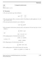
2.4 Summary
Further Reading
Exercises

5
5
5
7
7
8
10
10
11
11
12
13
13
20

21
21
22
23
23
23

3

Continuous Signals
3.1 Classification of Signals
3.1.1 Continuous Signals
3.1.2 Periodic and Aperiodic Signals
3.1.3 Energy and Power Signals

29
29
29
30
31


vi

Contents

3.2

3.3

3.4

4

3.1.4 Even- and Odd-symmetric Signals
3.1.5 Causal and Noncausal Signals
Basic Signals
3.2.1 Unit-step Signal
3.2.2 Unit-impulse Signal
3.2.3 Unit-ramp Signal
3.2.4 Sinusoids
Signal Operations
3.3.1 Time Shifting
3.3.2 Time Reversal
3.3.3 Time Scaling
Summary
Further Reading
Exercises

Time-domain Analysis of Discrete Systems
4.1 Difference Equation Model
4.1.1 System Response
4.1.2 Impulse Response
4.1.3 Characterization of Systems by their Responses to Impulse
and Unit-step Signals
4.2 Classification of Systems
4.2.1 Linear and Nonlinear Systems
4.2.2 Time-invariant and Time-varying Systems
4.2.3 Causal and Noncausal Systems
4.2.4 Instantaneous and Dynamic Systems

4.2.5 Inverse Systems
4.2.6 Continuous and Discrete Systems
4.3 Convolution–Summation Model
4.3.1 Properties of Convolution–Summation
4.3.2 The Difference Equation and Convolution–Summation
4.3.3 Response to Complex Exponential Input
4.4 System Stability
4.5 Realization of Discrete Systems
4.5.1 Decomposition of Higher-order Systems
4.5.2 Feedback Systems
4.6 Summary
Further Reading
Exercises

31
33
33
33
34
42
43
45
45
46
47
48
48
48
53
53

55
58
60
61
61
62
63
64
64
64
64
67
68
69
71
72
73
74
74
75
75


Contents

vii

5

79

80
80
81
82
83
83
83
83
85
87
88
88
89

6

Time-domain Analysis of Continuous Systems
5.1 Classification of Systems
5.1.1 Linear and Nonlinear Systems
5.1.2 Time-invariant and Time-varying Systems
5.1.3 Causal and Noncausal Systems
5.1.4 Instantaneous and Dynamic Systems
5.1.5 Lumped-parameter and Distributed-parameter Systems
5.1.6 Inverse Systems
5.2 Differential Equation Model
5.3 Convolution-integral Model
5.3.1 Properties of the Convolution-integral
5.4 System Response
5.4.1 Impulse Response
5.4.2 Response to Unit-step Input

5.4.3 Characterization of Systems by their Responses to Impulse
and Unit-step Signals
5.4.4 Response to Complex Exponential Input
5.5 System Stability
5.6 Realization of Continuous Systems
5.6.1 Decomposition of Higher-order Systems
5.6.2 Feedback Systems
5.7 Summary
Further Reading
Exercises
The Discrete Fourier Transform
6.1 The Time-domain and the Frequency-domain
6.2 Fourier Analysis
6.2.1 Versions of Fourier Analysis
6.3 The Discrete Fourier Transform
6.3.1 The Approximation of Arbitrary Waveforms with a Finite
Number of Samples
6.3.2 The DFT and the IDFT
6.3.3 DFT of Some Basic Signals
6.4 Properties of the Discrete Fourier Transform
6.4.1 Linearity
6.4.2 Periodicity
6.4.3 Circular Shift of a Sequence
6.4.4 Circular Shift of a Spectrum
6.4.5 Symmetry
6.4.6 Circular Convolution of Time-domain Sequences

91
92
93

94
94
95
96
97
97
101
101
102
104
104
104
105
107
110
110
110
110
111
111
112


viii

Contents

6.5

6.6

6.4.7 Circular Convolution of Frequency-domain Sequences
6.4.8 Parseval’s Theorem
Applications of the Discrete Fourier Transform
6.5.1 Computation of the Linear Convolution Using the DFT
6.5.2 Interpolation and Decimation
Summary
Further Reading
Exercises

113
114
114
114
115
119
119
119

7

Fourier Series
7.1 Fourier Series
7.1.1 FS as the Limiting Case of the DFT
7.1.2 The Compact Trigonometric Form of the FS
7.1.3 The Trigonometric Form of the FS
7.1.4 Periodicity of the FS
7.1.5 Existence of the FS
7.1.6 Gibbs Phenomenon
7.2 Properties of the Fourier Series

7.2.1 Linearity
7.2.2 Symmetry
7.2.3 Time Shifting
7.2.4 Frequency Shifting
7.2.5 Convolution in the Time-domain
7.2.6 Convolution in the Frequency-domain
7.2.7 Duality
7.2.8 Time Scaling
7.2.9 Time Differentiation
7.2.10 Time Integration
7.2.11 Parseval’s Theorem
7.3 Approximation of the Fourier Series
7.3.1 Aliasing Effect
7.4 Applications of the Fourier Series
7.5 Summary
Further Reading
Exercises

123
123
123
125
126
126
126
130
132
133
133
135

135
136
137
138
138
139
140
140
141
142
144
145
145
145

8

The Discrete-time Fourier Transform
8.1 The Discrete-time Fourier Transform
8.1.1 The DTFT as the Limiting Case of the DFT
8.1.2 The Dual Relationship Between the DTFT and the FS
8.1.3 The DTFT of a Discrete Periodic Signal
8.1.4 Determination of the DFT from the DTFT

151
151
151
156
158
158

Contents

8.2

8.3
8.4

8.5

9

ix

Properties of the Discrete-time Fourier Transform
8.2.1 Linearity
8.2.2 Time Shifting
8.2.3 Frequency Shifting
8.2.4 Convolution in the Time-domain
8.2.5 Convolution in the Frequency-domain
8.2.6 Symmetry
8.2.7 Time Reversal
8.2.8 Time Expansion
8.2.9 Frequency-differentiation
8.2.10 Difference
8.2.11 Summation
8.2.12 Parseval’s Theorem and the Energy Transfer Function
Approximation of the Discrete-time Fourier Transform
8.3.1 Approximation of the Inverse DTFT by the IDFT

Applications of the Discrete-time Fourier Transform
8.4.1 Transfer Function and the System Response
8.4.2 Digital Filter Design Using DTFT
8.4.3 Digital Differentiator
8.4.4 Hilbert Transform
Summary
Further Reading
Exercises

The Fourier Transform
9.1 The Fourier Transform
9.1.1 The FT as a Limiting Case of the DTFT
9.1.2 Existence of the FT
9.2 Properties of the Fourier Transform
9.2.1 Linearity
9.2.2 Duality
9.2.3 Symmetry
9.2.4 Time Shifting
9.2.5 Frequency Shifting
9.2.6 Convolution in the Time-domain
9.2.7 Convolution in the Frequency-domain
9.2.8 Conjugation
9.2.9 Time Reversal
9.2.10 Time Scaling
9.2.11 Time-differentiation
9.2.12 Time-integration

159
159
159

160
161
162
163
164
164
166
166
167
168
168
170
171
171
174
174
175
178
178
178
183
183
183
185
190
190
190
191
192
192

193
194
194
194
194
195
197


x

Contents

9.3

9.4
9.5

9.6

9.2.13 Frequency-differentiation
9.2.14 Parseval’s Theorem and the Energy Transfer Function
Fourier Transform of Mixed Classes of Signals
9.3.1
The FT of a Continuous Periodic Signal
9.3.2
Determination of the FS from the FT
9.3.3
The FT of a Sampled Signal and the Aliasing Effect
9.3.4

The FT of a Sampled Aperiodic Signal and the DTFT
9.3.5
The FT of a Sampled Periodic Signal and the DFT
9.3.6
Approximation of a Continuous Signal from its Sampled
Version
Approximation of the Fourier Transform
Applications of the Fourier Transform
9.5.1
Transfer Function and System Response
9.5.2
Ideal Filters and their Unrealizability
9.5.3
Modulation and Demodulation
Summary
Further Reading
Exercises

10 The z-Transform
10.1 Fourier Analysis and the z-Transform
10.2 The z-Transform
10.3 Properties of the z-Transform
10.3.1 Linearity
10.3.2 Left Shift of a Sequence
10.3.3 Right Shift of a sequence
10.3.4 Convolution
10.3.5 Multiplication by n
10.3.6 Multiplication by an
10.3.7 Summation
10.3.8 Initial Value

10.3.9 Final Value
10.3.10 Transform of Semiperiodic Functions
10.4 The Inverse z-Transform
10.4.1 Finding the Inverse z-Transform
10.5 Applications of the z-Transform
10.5.1 Transfer Function and System Response
10.5.2 Characterization of a System by its Poles and Zeros
10.5.3 System Stability
10.5.4 Realization of Systems
10.5.5 Feedback Systems

198
198
200
200
202
203
206
207
209
209
211
211
214
215
219
219
219
227
227

228
232
232
233
234
234
235
235
236
236
237
237
237
238
243
243
245
247
248
251


Contents

10.6 Summary
Further Reading
Exercises

xi

253
253
253

11 The Laplace Transform
11.1 The Laplace Transform
11.1.1 Relationship Between the Laplace Transform and the
z-Transform
11.2 Properties of the Laplace Transform
11.2.1 Linearity
11.2.2 Time Shifting
11.2.3 Frequency Shifting
11.2.4 Time-differentiation
11.2.5 Integration
11.2.6 Time Scaling
11.2.7 Convolution in Time
11.2.8 Multiplication by t
11.2.9 Initial Value
11.2.10 Final Value
11.2.11 Transform of Semiperiodic Functions
11.3 The Inverse Laplace Transform
11.4 Applications of the Laplace Transform
11.4.1 Transfer Function and System Response
11.4.2 Characterization of a System by its Poles and Zeros
11.4.3 System Stability
11.4.4 Realization of Systems
11.4.5 Frequency-domain Representation of Circuits
11.4.6 Feedback Systems
11.4.7 Analog Filters
11.5 Summary

Further Reading
Exercises

259
259
262
263
263
264
264
265
267
268
268
269
269
270
270
271
272
272
273
274
276
276
279
282
285
285
285

12 State-space Analysis of Discrete Systems
12.1 The State-space Model
12.1.1 Parallel Realization
12.1.2 Cascade Realization
12.2 Time-domain Solution of the State Equation
12.2.1 Iterative Solution
12.2.2 Closed-form Solution
12.2.3 The Impulse Response

293
293
297
299
300
300
301
307


xii

Contents

12.3 Frequency-domain Solution of the State Equation
12.4 Linear Transformation of State Vectors
12.5 Summary
Further Reading
Exercises

308
310
312
313
313

13 State-space Analysis of Continuous Systems
13.1 The State-space Model
13.2 Time-domain Solution of the State Equation
13.3 Frequency-domain Solution of the State Equation
13.4 Linear Transformation of State Vectors
13.5 Summary
Further Reading
Exercises

317
317
322
327
330
332
333
333

Appendix A: Transform Pairs and Properties

337

Appendix B: Useful Mathematical Formulas

349

Answers to Selected Exercises

355

Index

377


Preface
The increasing number of applications, requiring a knowledge of the theory of signals and systems, and the rapid developments in digital systems technology and fast
numerical algorithms call for a change in the content and approach used in teaching
the subject. I believe that a modern signals and systems course should emphasize the
practical and computational aspects in presenting the basic theory. This approach to
teaching the subject makes the student more effective in subsequent courses. In addition, students are exposed to practical and computational solutions that will be of use
in their professional careers. This book is my attempt to adapt the theory of signals
and systems to the use of computers as an efficient analysis tool.
A good knowledge of the fundamentals of the analysis of signals and systems is
required to specialize in such areas as signal processing, communication, and control.
As most of the practical signals are continuous functions of time, and since digital
systems are mostly used to process them, the study of both continuous and discrete
signals and systems is required. The primary objective of writing this book is to present
the fundamentals of time-domain and frequency-domain methods of signal and linear
time-invariant system analysis from a practical viewpoint. As discrete signals and
systems are more often used in practice and their concepts are relatively easier to
understand, for each topic, the discrete version is presented first, followed by the
corresponding continuous version. Typical applications of the methods of analysis
are also provided. Comprehensive coverage of the transform methods, and emphasis

on practical methods of analysis and physical interpretation of the concepts are the
key features of this book. The well-documented software, which is a supplement
to this book and available on the website (www.wiley.com/go/sundararajan), greatly
reduces much of the difficulty in understanding the concepts. Based on this software,
a laboratory course can be tailored to suit individual course requirements.
This book is intended to be a textbook for a junior undergraduate level onesemester signals and systems course. This book will also be useful for self-study.
Answers to selected exercises, marked ∗, are given at the end of the book. A Solutions
manual and slides for instructors are also available on the website (www.wiley.com/
go/sundararajan). I assume responsibility for any errors in this book and in the
accompanying supplements, and would very much appreciate receiving readers’ suggestions and pointing out any errors (email address: d ).

xiii


xiv

Preface

I am grateful to my editor and his team at Wiley for their help and encouragement in
completing this project. I thank my family and my friend Dr A. Pedar for their support
during this endeavor.
D. Sundararajan


Abbreviations
dc:
DFT:
DTFT:
FT:
FS:

IDFT:
Im:
LTI:
Re:
ROC:

Constant
Discrete Fourier transform
Discrete-time Fourier transform
Fourier transform
Fourier series
Inverse discrete Fourier transform
Imaginary part of a complex number or expression
Linear time-invariant
Real part of a complex number or expression
Region of convergence



1
Introduction
In typical applications of science and engineering, we have to process signals, using
systems. While the applications vary from communication to control, the basic analysis
and design tools are the same. In a signals and systems course, we study these tools:
convolution, Fourier analysis, z-transform, and Laplace transform. The use of these
tools in the analysis of linear time-invariant (LTI) systems with deterministic signals is
presented in this book. While most practical systems are nonlinear to some extent, they
can be analyzed, with acceptable accuracy, assuming linearity. In addition, the analysis
is much easier with this assumption. A good grounding in LTI system analysis is also
essential for further study of nonlinear systems and systems with random signals.

For most practical systems, input and output signals are continuous and these signals
can be processed using continuous systems. However, due to advances in digital systems technology and numerical algorithms, it is advantageous to process continuous
signals using digital systems (systems using digital devices) by converting the input
signal into a digital signal. Therefore, the study of both continuous and digital systems
is required. As most practical systems are digital and the concepts are relatively easier
to understand, we describe discrete signals and systems first, immediately followed
by the corresponding description of continuous signals and systems.

1.1 The Organization of this Book
Four topics are covered in this book. The time-domain analysis of signals and systems
is presented in Chapters 2–5. The four versions of the Fourier analysis are described in
Chapters 6–9. Generalized Fourier analysis, the z-transform and the Laplace transform,
are presented in Chapters 10 and 11. State space analysis is introduced in Chapters 12
and 13.
The amplitude profile of practical signals is usually arbitrary. It is necessary to
represent these signals in terms of well-defined basic signals in order to carry out
A Practical Approach to Signals and Systems
© 2008 John Wiley & Sons (Asia) Pte Ltd

D. Sundararajan


2

A Practical Approach to Signals and Systems

efficient signal and system analysis. The impulse and sinusoidal signals are fundamental in signal and system analysis. In Chapter 2, we present discrete signal classifications, basic signals, and signal operations. In Chapter 3, we present continuous
signal classifications, basic signals, and signal operations.
The study of systems involves modeling, analysis, and design. In Chapter 4, we
start with the modeling of a system with the difference equation. The classification

of systems is presented next. Then, the convolution–summation model is introduced.
The zero-input, zero-state, transient, and steady-state responses of a system are derived
from this model. System stability is considered in terms of impulse response. The basic
components of discrete systems are identified. In Chapter 5, we start with the classification of systems. The modeling of a system with the differential equation is presented
next. Then, the convolution-integral model is introduced. The zero-input, zero-state,
transient, and steady-state responses of a system are derived from this model. System stability is considered in terms of impulse response. The basic components of
continuous systems are identified.
Basically, the analysis of signals and systems is carried out using impulse or sinusoidal signals. The impulse signal is used in time-domain analysis, which is presented
in Chapters 4 and 5. Sinusoids (more generally complex exponentials) are used as the
basic signals in frequency-domain analysis. As frequency-domain analysis is generally more efficient, it is most often used. Signals occur usually in the time-domain. In
order to use frequency-domain analysis, signals and systems must be represented in
the frequency-domain. Transforms are used to obtain the frequency-domain representation of a signal or a system from its time-domain representation. All the essential
transforms required in signal and system analysis use the same family of basis signals,
a set of complex exponential signals. However, each transform is more advantageous
to analyze certain types of signal and to carry out certain types of system operations,
since the basis signals consists of a finite or infinite set of complex exponential signals
with different characteristics—continuous or discrete, and the exponent being complex or pure imaginary. The transforms that use the complex exponential with a pure
imaginary exponent come under the heading of Fourier analysis. The other transforms
use exponentials with complex exponents as their basis signals.
There are four versions of Fourier analysis, each primarily applicable to a different
type of signals such as continuous or discrete, and periodic or aperiodic. The discrete
Fourier transform (DFT) is the only one in which both the time- and frequency-domain
representations are in finite and discrete form. Therefore, it can approximate other
versions of Fourier analysis through efficient numerical procedures. In addition, the
physical interpretation of the DFT is much easier. The basis signals of this transform is
a finite set of harmonically related discrete exponentials with pure imaginary exponent.
In Chapter 6, the DFT, its properties, and some of its applications are presented.
Fourier analysis of a continuous periodic signal, which is a generalization of the
DFT, is called the Fourier series (FS). The FS uses an infinite set of harmonically
related continuous exponentials with pure imaginary exponent as the basis signals.

Introduction

3

This transform is useful in frequency-domain analysis and design of periodic signals
and systems with continuous periodic signals. In Chapter 7, the FS, its properties, and
some of its applications are presented.
Fourier analysis of a discrete aperiodic signal, which is also a generalization of the
DFT, is called the discrete-time Fourier transform (DTFT). The DTFT uses a continuum of discrete exponentials, with pure imaginary exponent, over a finite frequency
range as the basis signals. This transform is useful in frequency-domain analysis and
design of discrete signals and systems. In Chapter 8, the DTFT, its properties, and
some of its applications are presented.
Fourier analysis of a continuous aperiodic signal, which can be considered as a
generalization of the FS or the DTFT, is called the Fourier transform (FT). The FT
uses a continuum of continuous exponentials, with pure imaginary exponent, over an
infinite frequency range as the basis signals. This transform is useful in frequencydomain analysis and design of continuous signals and systems. In addition, as the
most general version of Fourier analysis, it can represent all types of signals and is
very useful to analyze a system with different types of signals, such as continuous or
discrete, and periodic or aperiodic. In Chapter 9, the FT, its properties, and some of
its applications are presented.
Generalization of Fourier analysis for discrete signals results in the z-transform.
This transform uses a continuum of discrete exponentials, with complex exponent,
over a finite frequency range of oscillation as the basis signals. With a much larger set
of basis signals, this transform is required for the design, and transient and stability
analysis of discrete systems. In Chapter 10, the z-transform is derived from the DTFT
and, its properties and some of its applications are presented. Procedures for obtaining
the forward and inverse z-transforms are described.
Generalization of Fourier analysis for continuous signals results in the Laplace

transform. This transform uses a continuum of continuous exponentials, with complex
exponent, over an infinite frequency range of oscillation as the basis signals. With a
much larger set of basis signals, this transform is required for the design, and transient
and stability analysis of continuous systems. In Chapter 11, the Laplace transform is
derived from the FT and, its properties and some of its applications are presented.
Procedures for obtaining the forward and inverse Laplace transforms are described.
In Chapter 12, state-space analysis of discrete systems is presented. This type of
analysis is more general in that it includes the internal description of a system in
contrast to the input–output description of other types of analysis. In addition, this
method is easier to extend to system analysis with multiple inputs and outputs, and
nonlinear and time-varying system analysis. In Chapter 13, state-space analysis of
continuous systems is presented.
In Appendix A, transform pairs and properties are listed. In Appendix B, useful
mathematical formulas are given.
The basic problem in the study of systems is how to analyze systems with arbitrary
input signals. The solution, in the case of linear time-invariant (LTI) systems, is to


4

A Practical Approach to Signals and Systems

decompose the signal in terms of basic signals, such as the impulse or the sinusoid.
Then, with knowledge of the response of a system to these basic signals, the response
of the system to any arbitrary signal that we shall ever encounter in practice, can be
obtained. Therefore, the study of the response of systems to the basic signals, along
with the methods of decomposition of arbitrary signals in terms of the basic signals,
constitute the study of the analysis of systems with arbitrary input signals.

2
Discrete Signals
A signal represents some information. Systems carry out tasks or produce output signals in response to input signals. A control system may set the speed of a motor in
accordance with an input signal. In a room-temperature control system, the power to
the heating system is regulated with respect to the room temperature. While signals
may be electrical, mechanical, or of any other form, they are usually converted to electrical form for processing convenience. A speech signal is converted from a pressure
signal to an electrical signal in a microphone. Signals, in almost all practical systems,
have arbitrary amplitude profile. These signals must be represented in terms of simple and well-defined mathematical signals for ease of representation and processing.
The response of a system is also represented in terms of these simple signals. In Section 2.1, signals are classified according to some properties. Commonly used basic
discrete signals are described in Section 2.2. Discrete signal operations are presented
in Section 2.3.

2.1 Classification of Signals
Signals are classified into different types and, the representation and processing of a
signal depends on its type.

2.1.1 Continuous, Discrete and Digital Signals
A continuous signal is specified at every value of its independent variable. For example, the temperature of a room is a continuous signal. One cycle of the continuous
π
2π
complex exponential signal, x(t) = ej( 16 t+ 3 ) , is shown in Figure 2.1(a). We denote a
continuous signal, using the independent variable t, as x(t). We call this representation the time-domain representation, although the independent variable is not time for
some signals. Using Euler’s identity, the signal can be expressed, in terms of cosine and
A Practical Approach to Signals and Systems
© 2008 John Wiley & Sons (Asia) Pte Ltd

D. Sundararajan


6

A Practical Approach to Signals and Systems

1

real

x(n)

x(t)

1
0

imaginary

−1
0

4

8
t

12

real

0
imaginary

−1

16

0

4

8
n

(a)

12

16

(b)
2π

π

Figure 2.1 (a) The continuous complex exponential signal, x(t) = ej( 16 t+ 3 ) ; (b) the discrete complex
π
2π
exponential signal, x(n) = ej( 16 n+ 3 )

sine signals, as
2π

π

x(t) = ej( 16 t+ 3 ) = cos

π
2π
t+
16
3

+ j sin

π
2π
t+
16
3

t + π3 ) and the imaginary part is the real
The real part of x(t) is the real sinusoid cos( 2π
16
sinusoid sin( 2π
t + π3 ), as any complex signal is an ordered pair of real signals. While
16
practical signals are real-valued with arbitrary amplitude profile, the mathematically
well-defined complex exponential is predominantly used in signal and system analysis.
A discrete signal is specified only at discrete values of its independent variable.
For example, a signal x(t) is represented only at t = nTs as x(nTs ), where Ts is the
sampling interval and n is an integer. The discrete signal is usually denoted as x(n),

suppressing Ts in the argument of x(nTs ). The important advantage of discrete signals is that they can be stored and processed efficiently using digital devices and
fast numerical algorithms. As most practical signals are continuous signals, the discrete signal is often obtained by sampling the continuous signal. However, signals
such as yearly population of a country and monthly sales of a company are inherently discrete signals. Whether a discrete signal arises inherently or by sampling, it
is represented as a sequence of numbers {x(n), −∞ < n < ∞}, where the independent variable n is an integer. Although x(n) represents a single sample, it is also used
to denote the sequence instead of {x(n)}. One cycle of the discrete complex expoπ
2π
nential signal, x(n) = ej( 16 n+ 3 ) , is shown in Figure 2.1(b). This signal is obtained
by sampling the signal (replacing t by nTs ) in Figure 2.1(a) with Ts = 1 s. In this
book, we assume that the sampling interval, Ts , is a constant. In sampling a signal,
the sampling interval, which depends on the frequency content of the signal, is an
important parameter. The sampling interval is required again to convert the discrete
signal back to its corresponding continuous form. However, when the signal is in
discrete form, most of the processing is independent of the sampling interval. For
example, summing of a set of samples of a signal is independent of the sampling
interval.
When the sample values of a discrete signal are quantized, it becomes a digital
signal. That is, both the dependent and independent variables of a digital signal are in