- Trang chủ >>
- Khoa Học Tự Nhiên >>
- Vật lý
Glenn f knoll complete solutions manual to Radi(BookZZ org)
Bạn đang xem bản rút gọn của tài liệu. Xem và tải ngay bản đầy đủ của tài liệu tại đây (7.2 MB, 141 trang )
Chapter 1 Solutions
Radiation Sources
� Problem 1.1. Radiation Energy Spectra: Line vs. Continuous
Line (or discrete energy): a, c, d, e, f, and i.
Continuous energy: b, g, and h.
� Problem 1.2. Conversion electron energies compared.
Since the electrons in outer shells are bound less tightly than those in closer shells, conversion electrons from outer shells will
have greater emerging energies. Thus, the M shell electron will emerge with greater energy than a K or L shell electron.
� Problem 1.3. Nuclear decay and predicted energies.
We write the conservation of energy and momentum equations and solve them for the energy of the alpha particle. Momentum is
given the symbol "p", and energy is "E". For the subscripts, "al" stands for alpha, while "b" denotes the daughter nucleus.
pal 2
pal � pb � 0
2 mal
� Eal
pb 2
2 mb
� Eb
Eal � Eb � Q
and
Q � 5.5 MeV
Solving our system of equations for Eal, Eb , pal, pb , we get the solutions shown below. Note that we have two possible sets of
solutions (this does not effect the final result).
Eb � 5.5 1 �
mal
Eal �
mal � mb
3.31662
pal � �
mal
mb
5.5 mal
mal � mb
3.31662
pb � �
mal � mb
mal
mb
mal � mb
We are interested in finding the energy of the alpha particle in this problem, and since we know the mass of the alpha particle and
the daughter nucleus, the result is easily found. By substituting our known values of mal � 4 and mb � 206 into our derived
Ealequation we get:
Eal � 5.395 MeV
Note : We can obtain solutions for all the variables by substituting mb � 206 and mal � 4 into the derived equations above :
Eal � 5.395 MeV
Eb � 0.105 MeV
pal � � 6.570
amu � MeV
pb � � 6.570
amu � MeV
� Problem 1.4. Calculation of Wavelength from Energy.
Since an x-ray must essentially be created by the de-excitation of a single electron, the maximum energy of an x-ray emitted in a
tube operating at a potential of 195 kV must be 195 keV. Therefore, we can use the equation E=h�, which is also E=hc/Λ, or
Λ=hc/E. Plugging in our maximum energy value into this equation gives the minimum x-ray wavelength.
Λ�
h�c
E
where we substitute h � 6.626 � 10�34 J � s, c � 299 792 458 m � s and E � 195 keV
1
Chapter 1 Solutions
Λ �
1.01869 J–m
� 0.0636 Angstroms
KeV
� Problem 1.5.
235
UFission Energy Release.
Using the reaction
235
U �
117
Sn � 118 Sn, and mass values, we calculate the mass defect of:
M �235 U� � �M �117 Sn� � M �118 Sn�� � �M
and an expected energy release of �Mc2 .
Q � �235.0439 � �116.9029 � 117.9016�� AMU �
931.5 MeV
� 223 MeV
AMU
This is one of the most exothermic reactions available to us. This is one reason why, of course, nuclear power from uranium
fission is so attractive.
� Problem 1.6. Specific Activity of Tritium.
Here, we use the text equation Specific Activity = (ln(2)*Av)/ �T1�2 *M), where Av is Avogadro's number, T1�2 is the half-life of
the isotope, and M is the molecular weight of the sample.
Specific Activity �
ln�2� � Avogadro ' s Constant
T1�2 M
We substitute T1�2 � 12.26 years and M=
Specific Activity �
3 grams
mole
to get the specific activity in disintegrations/(gram–year).
1.13492 � 1022
gram –year
The same result expressed in terms of kCi/g is shown below
Specific Activity �
9.73 kCi
gram
� Problem 1.7. Accelerated particle energy.
The energy of a particle with charge q falling through a potential �V is q�V. Since �V= 3 MV is our maximum potential
difference, the maximum energy of an alpha particle here is q*(3 MV), where q is the charge of the alpha particle (+2). The
maximum alpha particle energy expressed in MeV is thus:
Energy � 3 Mega Volts � 2 Electron Charges � 6. MeV
2
Chapter 1 Solutions
� Problem 1.8. Photofission of deuterium.
The reaction of interest is
2
1
D�
0
0
Γ � 10 n �
1
1
2
1
D�Γ�
1
0
n�
1
1
p + Q (-2.226 MeV)
p+ Q (-2.226 MeV). Thus, the Γ must bring an energy of at least 2.226 MeV
in order for this endothermic reaction to proceed. Interestingly, the opposite reaction will be exothermic, and one can expect to
find 2.226 MeV gamma rays in the environment from stray neutrons being absorbed by hydrogen nuclei.
� Problem 1.9. Neutron energy from D-T reaction by 150 keV deuterons.
We write down the conservation of energy and momentum equations, and solve them for the desired energies by eliminating the
momenta. In this solution, "a" represents the alpha particle, "n" represents the neutron, and "d" represents the deuteron (and, as
before, "p" represents momentum, "E" represents energy, and "Q" represents the Q-value of the reaction).
pa 2
pa � pn � pd
2 ma
pn 2
� Ea
2 mn
� En
pd 2
2 md
� Ed
Ea � En � Ed � Q
Next we want to solve the above equations for the unknown energies by eliminating the momenta. (Note : Using computer
software such as Mathematica is helpful for painlessly solving these equations).
We evaluate the solution by plugging in the values for particle masses (we use approximate values of "ma ," "mn ,"and "md " in
AMU, which is okay because we are interested in obtaining an energy value at the end). We define all energies in units of MeV,
namely the Q-value, and the given energy of the deuteron (both energy values are in MeV). So we substitute ma = 4, mn = 1, md
= 2, Q = 17.6, Ed = 0.15 into our momenta independent equations. This yields two possible sets of solutions for the energies (in
MeV). One corresponds to the neutron moving in the forward direction, which is of interest.
En � 13.340 MeV
En � 14.988 MeV
Ea � 4.410 MeV
Ea � 2.762 MeV
Next we solve for the momenta by eliminating the energies. When we substitute ma = 4, mn = 1, md = 2, Q = 17.6, Ed = 0.15 into
these equations we get the following results.
pn �
pd
5
�
1
2
5
3 pd 2 � 352
pa �
1
10
8 pd � 2
2
3 pd 2 � 352
We do know the initial momentum of the deuteron, however, since we know its energy. We can further evaluate our solutions for
pn and pa by substituting:
pd �
2 � 2 � 0.15
The particle momenta ( in units of
pn � �5.165
pn � 5.475
amu� MeV ) for each set of solutions is thus:
pa � 5.940
pa � �4.700
The largest neutron momentum occurs in the forward (+) direction, so the highest neutron energy of 14.98 MeV corresponds
to this direction.
3
Chapter 2 Solutions
Radiation Interaction Problems
� Problem 2.1 Stopping time in silicon and hydrogen.
Here, we apply Equation 2.3 from the text.
1.2 range
Tstop �
mass
energy
107
Now we evaluate our equation for an alpha particle stopped in silicon. We obtained the value for "range" from Figure 2.8
(converting from mass thickness to distance in meters by dividing by the density of Si � 2330 mg� cm3 ). The value for "mass" is
approximated as 4 AMU for the alpha particle, and the value for "energy" is 5 MeV.
We substitute
�6
range � 22 x 10 , mass � 4 and energy � 5 into Equation 2.3 to get the approximate alpha stopping time (in seconds) in silicon.
Tstop � 2.361 � 10�12 seconds
Now we do the same for the same alpha particle stopped in hydrogen gas. Again, we obtain the value for "range" (in meters)
from Figure 2.8 in the same manner as before (density of H � .08988 mg� cm3 ), and, of course, the values for "mass" and
"energy" are the same as before (nothing about the alpha particle has changed). We substitute range = 0.1, mass = 4 and energy
=5 into Equation 2.3 to get the approximate alpha stopping time (in seconds) in hydrogen gas.
Tstop � 1.073 � 10�8 seconds
The results from this problem tell us that the stopping times for alphas range from about picoseconds in solids to nanoseconds in
a gas.
� Problem 2.2. Partial energy lost in silicon for 5 MeV protons.
�Clever technique:
A 5 MeV proton has a range of 210 microns in silicon according to Figure 2-7. So, after passing through
100 microns, the proton has enough energy left to go another 110 microns. It takes about 3.1 MeV, according to the same figure,
to go this 110 microns, so this must be the remaining energy. Thus the proton must have lost 1.9 MeV in the first 100 microns.
� Problem 2.3. Energy loss of 1 MeV alpha in 5 microns Au.
From Figure 2.10, we find that
�1 dE
�
Ρ dx
380
MeV�cm2
.
g
Therefore,
dE
�
dx
380
MeV�cm2
*
g
Ρ (ignoring the negative sign will not
affect the result of this problem).
Energy loss �
We substitute dE �dx �
(in non-SI units).
4
Ρ �dE � dx� �x
Ρ
380 MeV cm2 Ρ
gram
, Ρ�
19.32 grams
cm3
and �x � 5 microns to get the energy loss of the 1 MeV Α-particle in 5 Μm Au
Chapter 2 Solutions
36 708 MeV microns
Energy loss �
cm
The result in SI units is thus:
Energy loss � 3.671 � 106 eV
Since this energy loss is greater than the initial energy of the particle, all of the Α-particle energy is lost before 5 Μm.
Note the small range of the Α , i.e. ~ Μm per MeV.
� Problem 2.4. Range of 1 MeV electrons in Al. Scaling Law.
The Bragg-Kleeman rule, or scaling law, allows us to relate the known range in one material to the range in another material.
The semi-empirical rule we use is:
R1
R0
�
Ρ0
A1
Ρ1
A0
(Equation 2.7)
Here, we use Figure 2.14 to approximate the 1 MeV electron range in silicon �R0 ), and since we know every other quantity in
Equation 2.7, we can approximate the range of the 1 MeV electron in aluminum �R1 ). Solving for
R1 we can find the estimated range of the electron in Aluminum.
AWAl
AWSi
rSi ΡSi
rAl �
We substitute rSi �
ΡAl
0.5 g
cm2 ΡSi
, AWAl � 26.9815 amu, AWSi � 28.0855 amu, ΡAl �
2.698 g
cm3
and ΡSi �
2.329 g
cm3
to get the approximate
range of 1 MeV electrons in aluminum (in cm).
rAl � 0.1816 cm
� Problem 2.5. Compton scattering.
This problem asks for the energy of the scattered photon from a 1 MeV photon that scattered through 90 degrees. We use the
Compton scattering formula (Equation 2.17). We write the Compton scattering formula, defining the scattering angle ("Θ") as 90
degrees and the photon energy ("E0 ") as 1 MeV.
Energy �
E0
�1�Cos���
E0
me � c2
�1
We substitute Θ = 90° and E0 � 1 MeV to get the energy of the scattered photon in MeV.
Energy � 0.338 MeV
� Problem 2.6. Prob of photoelectric in Si versus Ge
5
Chapter 2 Solutions
Problem 2.6. Prob of photoelectric in Si versus Ge
For a rough estimate, we can note that photoelectric probabilities vary as � Z 4.5 so we would expect that
ΤSi � ΤGe � � 14 � 32�
4.5
� 0.0242
� Problem 2.7. The dominant gamma ray interaction mechanism.
See Figure 2-20 and read off the answers (using the given gamma-ray energies and the Z-number for the given absorber in each
part).
Compton scattering: a, b, and d.
Photoelectric absorption: c
Pair production: e
� Problem 2.8. Mean free path in NaI of 1 MeV gamma-rays.
(a). The gamma-ray mean free path (Λ) in NaI is 1 � Μ ( where Μ is the total linear attenuation coefficient in NaI). The mass
attenuation coefficient ( ) is 0.06 cm2 � gm at 1 MeV according to Figure 2.18, and the density of NaI relative to water (Ρ) is
Μ
Ρ
1
3.67 gm� cm3 (by the definition of specific gravity). Therefore, we have Λ = 1 � Μ = Μ
Ρ
�Ρ
. Here, we will denote the mass
Μ
attenuation coefficient ( ) by Μ Ρ , so we have
Ρ
Λ�
1
�Μ Ρ Ρ�
We substitute Μ p �
0.06 cm2
g
and Ρ �
3.67 g
cm3
to get the mean free path of 1 MeV gamma-rays in NaI (in cm).
Λ � 4.54 cm
(b). Any photon which emerges from 1 cm cannot have undergone a photoelectric absorption. Neglecting buildup factors, the
probability that a photon emerges from the slab without having an interaction is e�ΜT x , where ΜT is the total attenuation coeffiinteraction (1-e�ΜT x ). The probability that the interaction is a photoelectric interaction is Τ � ΜT (this is not the probability per unit
cient. The complement of this is the probability that a photon doesn't emerge from the slab without having had at least one
photon undergoes photoelectric absorption in the slab is (Τ � ΜT )*(1-e�ΜT x ). This equation is expressed below, along with the
path length, but the total probability that any given interaction is a photoelectric interaction). Therefore, the probability that a
values for ΜT (which is just 1 divided by the previous result for Λ), the attenuation distance (denoted "x" and which is 1 cm), and
Τ, which is just the mass attenuation coefficient for photoelectric absorption (found on Figure 2.18 to be 0.01) multiplied by the
density of NaI (3.67 g/cm3).
Probability of photoelectric absorption �
We substitute ΜΤ �
�
1 cm NaI.
6
1
,
4.54 cm
x � 1 cm and Τ �
0.01�3.67
cm
Τ �1 � ��ΜΤ x �
Μ
to get the probability of photoelectric absorption for 600 keV gamma-rays in
Chapter 2 Solutions
We substitute ΜΤ �
1
,
4.54 cm
x � 1 cm and Τ �
0.01�3.67
cm
to get the probability of photoelectric absorption for 600 keV gamma-rays in
1 cm NaI.
Probability of photoelectric absorption � 0.0329
What is interesting is that a different result is obtained using a different, although seemingly equally valid approach. We can note
that the probability per unit path length of a photoelectric interaction is Τ, so 1 � e�Τx is the probability of a photoelectric interaction in traveling a distance x.
Probability of a photoelectric interaction � 1 � ��Τ x
We substitute x=1cm and Τ=
0.010�3.67
to
cm
get the probability of a photoelectric interaction in traveling a distance x.
Probability of a photoelectric interaction � 0.0360
This result is slightly (10%) larger from the previous answer because this approach does not account for the attenuation of
photons through the material by other means.
� Problem 2.9. Definitions
See text.
� Problem 2.10. Mass attenuation coefficient for compounds.
The linear attenuation coefficient is the probability per path length of an interaction. In a compound, the total linear attenuation
coefficient would be given by the sum over the ith constituents multiplied by the density of the compound:
Μc = Ρc �wi � Ρ �
Μ
(Equation 2.23)
i
where wi is the weight fraction of the ith constituent in the compound (represented by "wH " and "wO ," respectively, in this problem), �Μ � Ρ�i is the mass attenuation coefficient of the ith constituent in the compound (represented by "ΜH " and "ΜO ," respec-
tively), and Ρc is the density of the compound (represented by "ΡW " for the density of water). The expression below shows this
sum for water attenuating 140 keV gamma rays:
Μc � ΡW �ΜH wH � ΜO wO �
We substitute ΜH � .26 cm2 � g, ΜO � .14 cm2 � g, ΡW � 1 g � cm3 , wH � 2 � 18 and wO � 16 �18 to get the linear attenuation
coefficient for water attenuating 140 keV gamma rays.
Μc �
0.153333
cm
The mean free path, Λ, is just the inverse of this last calculated value, or
1
. The mean free path of 140 keV gamma rays in
ΜC
water is thus:
ΛH2 O � 6.52 cm
This turns out to be an important result because Tc � 99 m is a radioisotope routinely used in medical diagnostics and it emits
140 keV gamma rays. Since most of the human body is made of water, this gives us an idea of how far these gamma rays can
travel without an interaction through the human body and into our detectors.
7
Chapter 2 Solutions
This turns out to be an important result because Tc � 99 m is a radioisotope routinely used in medical diagnostics and it emits
140 keV gamma rays. Since most of the human body is made of water, this gives us an idea of how far these gamma rays can
travel without an interaction through the human body and into our detectors.
� Problem 2.11. 1 J of energy from 5 MeV depositions.
We are looking for the number of 5 MeV alpha particles that would be required to deposit 1 J of energy, which is the same as
looking for how many 5 MeV energy depositions equal 1 J of energy. We expect the number to be large since 1 J is a macroscopic unit of energy. To find this number, we simply take the ratio between 1 J and 5 MeV, noting that 1 MeV = 1.6 x 10�13 J .
The number of 5 MeV alpha particles required to deposit 1 J of energy is thus:
n�
1 Joule
� 1.25 � 1012 alpha particles
5 MeV
� Problem 2.12. Beam energy deposition.
100 ΜA tells us the current, i.e., the number of Coulombs passing in unit time. If we divide this by the amount of charge per
particle, it gives us the number of particles passing through the area in unit time. If we take this value, and multiply it by the
energy per particle, we get the energy/time, or power. The power dissipated in the target by a beam of 1 MeV electrons with a
current of 100 ΜA is thus:
Power �
�100 ΜA� �1 MeV�
�Electron Charge�
� 100 Watts
This is a surprisingly low amount of power, about the same as from a light bulb, and represents the output from a small accelerating device.
� Problem 2.13. Exposure rate 5 m from 1 Ci of
60
Co.
We use the following equation for exposure rate:
Exposure Rate = �s
Α
d2
(Equation 2.31)
where Α is the source activity, d is the distance away from the source, and �s is the exposure rate constant. The exposure rate
constant for Co-60 is 13.2 R � cm2 � hr � mCi (from Table 2.1). The exposure rate 5 m from a 1 Ci Co-60 source is thus:
Exposure Rate � �s
Exposure Rate �
Α
d2
where we substitute Α � 1 Ci, d � 5 m, �s � 13.2
0.528 cm2 R
hr mm2
�
52.8 mR
The result in SI units :
Exposure Rate �
3.78 � 10�9 C
kg � s
� Problem 2.14. �T/�t from 10 mrad/hr.
8
hr
R � cm2
hr � mCi
Chapter 2 Solutions
Problem 2.14. �T/�t from 10 mrad/hr.
The dose of 1 rad corresponds to an energy deposition of 100 ergs/gram. So 10 mrad/hr corresponds to 1 erg/(gram-hr). Using a
specific heat of water as 1 calorie � �gram �o C), we can use the equation �Q � mC p �T. Our given 1 ergs/(gram-hr) is
�Q/(m*�t). If we divide our equation by mC p , we are left with �T/�t on the right side, which is the quantity of interest, i.e.
�T/�t =
�Q��m�t�
Cp
�T
�t
�
=
1 ergs��gram�hr�
.
1 calorie��gram �o C�
1 Erg
1 Gram Calorie Hour
Gram Centigrade
The result below is the rate of temperature rise in a sample of liquid water with an absorbed dose rate of 10 mrad/h. Note that
this is virtually impossible to measure because it is so small.
�T
�t
�
2.39 � 10�8 Centigrade
Hour
There are unusual radiation detectors which actually use the temperature rise in a detecting material to detect ionizing radiation.
For the curious reader, do some research on bolometers in radiation detection, and also read about the superconducting radiation
detectors under development.
� Problem 2.15. Fluence-dose calculations for fast neutron source.
The Cf source emits fast neutrons with the spectrum N(E) dE given in the text by Eqn. 1.6. Each of those neutrons carries a dose
h(E) that depends on its energy as shown in Fig. 2.22(b). To get the total dose, we have to integrate N(E)h(E) over the energy
range.
First, let's consider only the neutron dose h(E). In the MeV range, we need a linear fit to the log h-log E plot of Figure 2.22(b) by
using two values read off the curve:
Log10 �10�12 � � b � m Log10 �0.01�
Log10 �10�10 � � b � m Log10 �1.0�
Solving the system of equations above yields :
m � 1 and b � �10
This result gives us an approximate functional form for h(E) �in Sv � cm2 �= 10�10 E �MeV�. Recall 1 Sv = 100 Rem = 105 mrem.
In a moment, we'll integrate N(E)h(E) to get the total dose-area, but first check the normalization of N(E):
norm � �
�
E �
�
E
1.3
�E
� 1.31359
0
We'll need this normalization factor because we will want to use N(E)/norm as the probability that a source neutron has energy E.
Now, a source neutron � cm2 arriving at the person delivers a dose (in Sv) of:
�0 E3�2 �
�
neutron � dose �
10
�
E
1.3
�E
� 1.95 � 10�10 Sv
10 norm
�We now need to multiply this by the number of neutrons produced by 3 micrograms of Cf-252 (2.3 x 10⁶ n/sec-mg) at 5 meters
over 8 hours:
9
Chapter 2 Solutions
We now need to multiply this by the number of neutrons produced by 3 micrograms of Cf-252 (2.3 x 10⁶ n/sec-mg) at 5 meters
over 8 hours:
dose � equivalent �
2.3 � 106 �3 Μg� �8 � 3600 sec�
Μ g sec� 4 Π 5002 �
� 63 254.5 neutrons � cm2
So the total dose equivalent is given by (using 105 mrem/Sv):
dose equivalentneutrons � 1.23 mrem
This is a small dose, comparable to natural background.
Aside: What about the dose from the gamma rays? They are high-energy gammas and the source emits 9.7 gammas per fission.
Using a value of hE ~ 5 x 10�12 Sv � cm2 :
dose equivalent Γ �
�2.3 � 106 neutrons� �3 Μg� �8 � 3600 sec� �5 Sv cm2 � �100 Rad� �1000 mRad�
�1 Μg sec� �1012 neutrons� �4 Π 500 cm2 � �Sv Rad�
� 0.0316 mRad
So the gamma dose is even smaller than that from the fast neutrons, as expected. Fast neutrons have a high quality factor, i.e.,
they produce a heavy charged particle when they interact, and therefore do a lot more biological damage than the light electrons
produced when gamma rays interact in materials.
10
Chapter 3 Solutions
Counting statistics problems
� Problem 3.1. Effect of increasing number of trials on sample variance.
The relative variance of the variable x, i.e.,
Σx 2
�x�
�
�x2 �
�x�2
� 1, is dependent only on the ratio of the means of x2 and x. It does not
depend upon the uncertainty in those quantities. Since these means are not expected to change with more samples, the relative
variance (i.e., 2% of the mean) shouldn't change. Note that this conclusion is independent of the type of distribution (Poisson,
Guassian, Binomial, etc.) for x. However, for any quantity that is derived from measurements, such as the mean <x>, the
uncertainty in that quantity improves with additional measurements as shown by: Σ�x� �
�x�
N
.
� Problem 3.2. Probability of 8 heads occuring in 12 coin tosses.
We define the binomial distribution for n = 12 (12 trials), p = 0.5 (probability of a success is 1/2), and we give the value k = 8
(the number of successes we are interested in). We substitute the known values of n,p and k and evaluate the binomial distribution below to get the probability that exactly 8 heads (or tails for that matter) will occur in 12 tosses of a coin.
Probability �
n�
k � �n � k� �
pk �1 � p�n�k � 0.121
� Problem 3.3. Statistics of males occuring in random population samples.
The mean is well known to be (prob of success)*(number of trials) =0.75 N The probability of success of any one trial (drawing
a male) is large (so Poisson statistics is not valid) and the sample size is only 15. Binomial statistics therefore apply. We substitute n = 15 and p = 0.75 in the equations below to find the mean (x), variance ( Σ2 ) and standard deviation (Σ).
x � n � p � 11.25
Σ2 � n p �1 � p� � 2.81
Σ�
Σ2 �
n p �1 � p� � 1.68
� Problem 3.4. Probability of no sixes in ten rolls of a dice.
Here, we define our probability distribution function as a binomial distribution with n=10 (number of trials), p=1/6 (probability of
a success), and evaluating it at k=0 successes, which is the same as finding the probability that no sixes (or no fives, or fours,
etc.) will turn up in ten rolls of the dice. The probability that no sixes will turn up in ten rolls of a dice is thus:
Probability �
n�
k � �n � k� �
pk �1 � p�n�k � 0.162
11
Chapter 3 Solutions
� Problem 3.5. Statistics of errors in computer program statements.
Poisson statistics applies to this problem because the probability of success (an error) is low, but the expected number of successes is not >~20 (the expected number of successes is 250/60 � 4.17, so we cannot apply Gaussian statistics).
a) Here, we simply define the expected mean and standard deviation of a Poisson distribution with an expected number of
�
successes (x = np) of 250/60. Of course, the expected number of successes is the same as the expected mean (they are both equal
to np), and in Poisson statistics, the standard deviation is the same as the square root of the expected mean. This is reflected in
the results shown below:
x �
250
� 4.17
60
Σ�
x � 2.04
�
b) Next, we define a Poisson distribution with x= 100/60 (expected number of successes), and evaluate the Poisson probability
distribution function at k=0 successes. The probability that a 100-statement program will be free of errors is thus:
Probability �
��x x k
k�
� 0.189
� Problem 3.6. When is square-root of a number an estimate of uncertainty?
The only time the square root of a number is an estimate of its uncertainty is when the number is a direct sample of a population.
For example, the number cannot have units associated with it (i.e. the square root of a value is not an estimate of its uncertainty
when it is not a number of counts obtained by direct measurement).
(a). Yes. This is just a number of counts.
(b). Yes. This is just a number of counts.
(c). No. This is a processed number. One must use error propagation to determine the error in the quantity derived from the
measurements.
(d). No. A rate has units and involves a division of the number of counts by time. In this case, error propagation says: Σ2 =
N
T2
.
Σ = x � N where x is the expected value and N is the number of samples in the average.
(f). Yes. Although this is a processed quantity, it would yield the same result as if we had just counted for one 5 minute period.
Using error propagation: Σ = Sqrt �N1 �N2 + ... + N5 ), so the error in the sum is just square root of the sum. This only works for
sums, and not for subtractions.
(e).
No. An average is a processed quantity derived from the measured values. Error propagation says:
� Problem 3.7. Source + Background -> Net counts and uncertainty
We are asked to find net = (S+B) - B and Σnet . Finding Σnet is a straight forward error propagation since all counts are taken for 1
minute. Below we define the equation for the net counts and the standard error propagation formula (Eqn. 3.37). As a shorthand
notation, the error propagation equation is expressed as a dot product between the two vectors representing the squared partial
derivativies and the corresponding variances. The variable "sb" refers to (S+B) and "b" refers to B in the equation for "net".
net � sb � b
12
Chapter 3 Solutions
�
Σnet �
� net
� sb
� net
2
,
�b
2
�.�Σsb 2 , Σb 2 �
We substitute sb=561, b=410, Σsb 2 � sb and Σb 2 � b to get the net number of counts and the expected uncertainty in the net
number of counts (Σnet ).
net � 151 counts
Σnet � 31.16
� Problem 3.8. Source + Background -> Net count rate and uncertainty
In this problem, the source plus background count rate (S+B) is 846 counts in 10 min, and the background count rate (B) is 73
counts in 10 min. We want the net count rate and its associated standard deviation. The net count rate is simply (S+B)-B, which
is calculated below.
net count rate �
846 � 73
�
77.3 counts
10
minute
The expected error, or the standard deviation, in the count rates for (S+B) and B are calculated using the error propagation
formula for division by a constant (Eq. 3.40), and then the standard deviation in the net count rate is calculated using error
propagtion for differences of counts (Eq. 3.38), where ΣS�B and ΣB are substituted for Σx and Σ y . The expected error, or standard
deviation, in the net count rate (counts/min) is thus:
Σnet �
846 � 73
10
�
3.03 counts
minute
� Problem 3.9. Results using optimal counting times for Problem 3.8.
We first solve the equation giving the optimal division of time (Eq. 3.54). This is done below, where we have again defined the
variables "sb" to denote the total counts of (S+B), and "b" to denote the background B in the equation. First we solve the system
of equations for Tsb and Tb , and then we substitute the measured values for the count rates (84.6 and 7.3 counts/min, respectively)
and the total amount of time allowed for the measurements to be done (20 min) to find the numerical values of Tsb and Tb .
sb
Tsb �
b
Tb
Tb � Tsb � Ttot
The resulting solutions for Tsb and Tb solved from the equations above is thus:.
sb
b
Ttot
Tsb �
Tb �
sb
b
�1
Ttot
sb
b
�1
We substitute sb = 84.6, b = 7.3 and Ttot � 20 to get the numerical values of Tsb and Tb in minutes (i.e. the optimal times for
measuring (S+B) and B, respectively).
13
Chapter 3 Solutions
Tsb � 15.46 minutes
Tb � 4.54 minutes
We now calculate the uncertainty in the net count rate using error propagation. When defining the net count rate, we denote the
number of counts over the new optimal time intervals as "nsb " and "nb ," respectively, and the optimal counting times as "tsb " and
"tb ," respectively. We then use the basic formula for error propagation with the appropriate variables (as in problem 3.7, the dot
between the two bracketed quantities signifies the dot product between the two, just as if we thought of them as two vectors).
Next we substitute in known values to get the expected error in the net count rate.
net �
nsb
�
tsb
nb
tb
Σnet count rate �
�
� net
� net
2
,
� nsb
2
� nb
�.�Σnsb 2 , Σnb 2 �
We substitute Σnsb 2 � nsb � 84.6 tsb , Σnb 2 � nb � 7.3 tb , tsb � 15.5 and tb � 4.5 to get the expected uncertainty in the net count
rate when the optimal time intervals are used.
Σnet count rate � 2.66
The improvement factor is thus 3.03/2.66.
� Problem 3.10. Counting time versus uncertainty.
We are looking for the improvement in the relative uncertainty of a measurement by longer counting. We know:
ΣN
N
�
N
N
�
1
1
�
N
, where N is the number of counts, R is the count rate, and T is the measurement time interval.
RT
Since we have only one measurement, N is assumed to be our experimental mean (see Eq. 3.29). Since the count rate remains
constant �R1 = R0 , and
Σ 2
�� NN �
T� =
1
1
= R1 ), we have :
R1
0
Σ 2
�� NN �
We already know that
[
�
T�
or
0
ΣN
�
N 0
Σ
� NN �
1
T1 = T0 �
] = � 2.8
�, and that T
1.0
0
�
2
ΣN
�
N 0
�
Σ
� NN �
1
= 10 min. From here, calculating T1 is very simple. The new counting time
in minutes is thus:
counting time � 10
2.8
2
� 78.4 minutes
1.0
Since the original counting time was 10 minutes, 68.4 minutes must be added to reduce the statistical uncertainty from 2.8%
to 1.0%.
14
Chapter 3 Solutions
� Problem 3.11. Better to increase source or decrease background?
Recall our relationship that the relative uncertainty (fractional standard deviation squared, or Ε2 ) in the source is given by:
1 � S�B �
T
S2
B�
2
(from Eqn. 3.55)
(a). If the S >> B, then this becomes
1
.
ST
Doubling the source strength is the best choice since the background is nearly irrele-
vant.
(b). If S << B, then this becomes
4B
. Doubling source improves the ratio by 4 times, whereas halving background only
S2 T
improves ratio by 2 times. Doubling the source strength is again the best choice.
� Problem 3.12. Probabilities of getting desired counts.
The expected number of counts in two minutes is (2 min)*(2.87 counts/min) = 5.74 counts. This is too small to apply Gaussian
statistics, so we assume Poisson statistics to be accurate.
a) Here, we define a Poisson distribution with a mean of 5.74 (or 2.87*2) counts (since this is the only measurement made), and
we use the Poisson probability density function (PDF):
Probability �
��Μ Μk
k�
We substitute Μ=5.74 and k=5 successes (i.e., counts) to get the probability that a given 2 minute count will contain exactly 5
counts.
Probability � 0.167
b) In order to determine the probability that at least one count will be recorded, we simply subtract the probability of 0 counts
being recorded from 1 (since the integral of the probability distribution function from 0 to infinity is normalized to 1).
Probability � 1 �
��Μ Μk
k�
We substitute Μ=5.74 and k=0 to get the probability that a given 2 minute count will contain at least 1 count:
Probability � 0.997
For the last part, we want to know how many counts are needed to ensure at least one count with probability >99%. Note that this
is the same as looking for the measurement time "t" required to acheive this number of counts (i.e. number of counts = (2.87
counts/min)*t). The key to this problem is to note that the probability of 0 counts must be less than 1% to satisfy this condition.
We again define our Poisson Distribution, but this time with a mean value of 2.87*t. We define the probability of observing no
counts to be 1%, and we solve for the resulting value for "t" that satisfies this condition:
��Μ Μk
k�
� .01
We substitute Μ=2.87t and k=0 then solve for t to get the minimum counting time required (in minutes) to ensure with > 99%
probability that at least one count is recorded:
15
Chapter 3 Solutions
t � 1.61 minutes
� Problem 3.13. Percent standard deviation between the activity ratio of two sources.
The ratio of the activity of Source B to Source A is simply given by:
Ratio =
��Source B�background count rate���background count rate��
��Source A�background count rate���background count rate��
This is represented below where we denote the number of counts by "c," measurement time by "t," background by "b," Source B
+ background by "bb," and Source A + background by "ab."
Ratio R �
cbb
tbb
�
cb
tb
cab
tab
�
cb
tb
We substitute cab � 251, tab � 5, cbb � 717, tbb � 2, cb � 51 and tb � 10 to get the ratio of the activity of Source B to Source A.
Ratio R � 7.84
Next, we define the explicit error propagation formula with the appropriate variables (as in previous problems, using the dot
product notation under the square root) and give the known values in counts and minutes, respectively.
Σ�
�
�R
� cab
�R
2
,
� cbb
�R
2
,
� cb
2
�.�cab , cbb , cb �
We substitute cab � 251, tab � 5, cbb � 717, tbb � 2, cb � 51 and tb � 10 to get the percent standard deviation in the ratio of the
activity of Source B to Source A.
ΣB�A � 0.635
� Problem 3.14. Estimating source measurement time based on desired error.
This problem is asking us to find the minimum measurement time interval necessary for the (source + background) counting rate
measurement such that the fractional standard deviation of the net source counting rate (source alone) is at most 3%. To do this,
we simply write the equation for the fractional standard deviation, set it equal to .03, and solve for the unknown time interval for
the source + background.
Below, we define the net counting rate as "R," "c" denotes a number of counts, "t" denotes a measurement time interval, "sb"
indicates a measurement for source + background, and "b" indicates a measurement for background. Next we define the fractional standard deviation for "R" (which is
ΣR
)
R
using the explicit form of the error propagation formula in the numerator in dot
product notation, as in previous problems. We then set
R�
csb
tsb
16
�
cb
tb
ΣR
R
equal to .03, substitute in known values and solve for tab .
Chapter 3 Solutions
�� �c � , � �c � �.�csb , cb �
�R 2
ΣR
sb
�R 2
b
�
� 0.03
R
R
We substitute csb � 80 tab , cb � 845 and tb � 30 then solve the above equation to get the time interval the source should be
counted for (with background) to determine the counting rate due to the source alone to within a fractional standard deviation of
3% (in minutes).
tab � 54.1 minutes
� Problem 3.15. Uncertainty in groups of measurements.
(a). The data fluctuations are expected to be statistical if the standard deviation of the sample population is the square root of the
mean. This seems true, but we check this with a Chi-squared distribution to be sure.
Here, we define the student's data set and calculate the standard deviation of that data set.
data � �25, 35, 30, 23, 27�
Σ � 4.69
Next, we take the square root of the mean (which is 28).
x � 5.29
Here, we define chi-squared ( Χ2 ) for the data set (using Eqn. 3.36).
Χ2 �
�N � 1� Σ2
x
We substitute N=5, Σ2 =22 and x=28 to get the value of Χ2 for our data set.
Χ2 �
22
7
�ni�1 x2i , where the xi are random variables
This is our "measured" value of Χ2 . One can also calculate the expected value of Χ2 from data values drawn from a predicted
distribution. (The Χ2 distribution is defined as the distribution of the quantity
following a normal distribution that has a unit variance and a mean value of zero).
To be consistent with the approach taken in the textbook, we actually want to calculate 1 minus the Χ2 "Cumulative Distribution
Function" (CDF). The Χ2 CDF is the integral from zero up to some argument, which in this case is
gives the probability that the expected value of Χ
2
22
.
7
The function CDF(x)
ranges between 0 and the value x, assuming the data follow the normal
distribution. The complement of this is then the probability that the expected value of Χ2 is larger than this value, which is what
the textbook uses. One can look these values up in statitics tables, but we use Mathematica to do this calculation for us:
1 � CDF� Χ2 4 degrees � of � freedom,
22
7
� � 0.534
Because this value is close to 0.5, the data are random (i.e. a true Poisson distribution would have a Χ2 probability of 0.5). As a
side note, this probability could also have been estimated using the Χ2 distribution table.
b) This question is asking that since the data appears to be random, what is the EXPECTED standard deviation of the MEAN of
�
5 single measurements using just these data. For this data set, given a mean , Σx� =
x
N
(Eqn. 3.44).
17
Chapter 3 Solutions
b) This question is asking that since the data appears to be random, what is the EXPECTED standard deviation of the MEAN of
�
5 single measurements using just these data. For this data set, given a mean , Σx� =
x
N
(Eqn. 3.44).
Using the provided data, the expected standard deviation in the mean of the data set is:
Σx �
x
� 2.37
N
(c). Now, suppose we have the 30 measurements of the mean from the 30 students. What would we expect to measure for the
variance of the set of these mean values �x1 , x2 , x3 ,.., x30 }?
The variance estimated in (b) above IS the expected fluctuation when samples are drawn identically from that population. So we
expect that the 30 mean values WILL show this variance (i.e. we would expect the sample variance in this situation to be the
result above squared, or s2 = Σ2 ; this is calculated to be � 5.59).
x
(d). Suppose we now average these 30 values to get a better estimate of the mean. What is the standard deviation for the mean?
One way to look at this is to see it as 5 x 30 data points and calculate Σx . The standard deviation goes down by
30 , so the
expected standard deviation of the mean when we use all 30 mean values will be 0.432049.
Another way is to calculate the standard deviation of the average of the averages. If we define
Σ�x� =
�x�
N
which, of course, turns out to be exactly the same formula.
18
Chapter 3 Solutions
� Problem 3.16. Chi-squared test on a data set of counting measurements.
Define the data set we are applying the chi-squared ( Χ2 ) test to as the variable "data":
data = {3626, 3731, 3572, 3689, 3625, 3711, 3617, 3572, 3578, 3569, 3677, 3630, 3615, 3605, 3591, 3678, 3624, 3652, 3595,
3636, 3465, 3574, 3601, 3540, 3629}
�
We determine the Χ2 value of the data by using the data values to calculate the sample variance (s2 ) and the sample mean x, and
then calculate:
Χ2data �
�No. of data values�1� Variance �data�
Mean �data�
Using a calculator to determine the mean and variance of the data set, one finds the mean is 3616.08 and Χ2 is 21.2191.
In problem 3.15(a) above, we described how to determine the probability that a true Poisson distribution would have fluctuations
larger than the data set by using the complement to the cumulative probability function of the Χ2 distribution.
We used Mathematica to calculate this probability, but it can also be found in your textbook or in standard tables of probabilities.
1 - CDF[ChiSquareDistribution(No. of data points - 1, Χ2 data )] = 0.626
Since this Χ2 probability is close to 0.5, the fluctuations are consistent with random fluctuations (relatively close to a true
Poisson distribution). In general, one looks for values that are very small (~5%) or very large (~95%) to indicate that the data
is not following the expected statistical model. If this is the case, then one looks at whether there is a problem with the
measurement system.
19
Chapter 3 Solutions
� Problem 3.17. Uncertainty in the difference between two measurements.
Suppose we are given that a set of I counts �Ni }, each taken over a period of time tI results in an average rate � r>. The uncertainty in the average rate can be determined from error propagation once we write the average rate in terms of the measured
counts:
<r> = (1/I)(N1 � tI � N2 �tI � ... NI �tI � � �1 � ItI � �N1 � N2 � ... NI � � Ntotal �ttotal
so
Σ�r� 2 � �1 �ItI �2 �N1 � N2 � ... � NI � � Ntotal � ttotal 2
We know that the total number of counts Ntotal � � r � ttotal . Since for this problem, we are given <r> and ttotal for each group,
we can find Ntotal for each group.
Wtih N A and NB ( total counts from Group A and Group B), we want to find out if the difference between � r � A and � r �B is
significant. Define this difference as:
�=
NA
TA
-
NB
.
TB
where T A is the total time for Group A (i.e., I * tI ), and similarly for Group B.
Using error propagation on these independent measurements,
Σ� 2 = �
� + � T B � � � � r A � � T A � � rB � � TB �, since ΣN A 2 � N A (i.e., the standard deviation in a number of counts is equal to
ΣN A 2
TA
Σ
2
B
the square root of that number).
If both groups are making identical measurements, we expect the probability of observing a given value of �, i.e., P(�), to be
Gaussian with <�>=0 and Σ� �
� r � �T �
1
A
1
�
TB
We look at our measured value of �, and see if it lies within � Σ� of 0. We will look at
�meas
and
Σ�theory
if this value is >> 1, then the
difference is significant since the probability of observing our value of � would be small.
Below we define
�
Σ�
�
�
,
Σ�
and substitute the known values for "N A ," "NB ," "T A ," and "TB "
NA
TA
�
NA
T A2
NB
TB
�
NB
TB2
We substitute N A � 2162.4 � 10, NB � 2081.5 � 20, T A � 10 and TB � 20 to get the value of
�
Σ�
�
.
Σ�
� 4.52
Since the difference between the two measured averages is 4.5 standard deviations from the expected mean (of zero), the difference is significant (i.e. there is a very small probability of observing such a value). We conclude that the premise that both
groups were making the same measurement is highly unlikely.
� Problem 3.18. Optimal total counting time in source activity calibration.
20
Chapter 3 Solutions
Problem 3.18. Optimal total counting time in source activity calibration.
This problem is solved based on the assumption that if both sources are counted for the same amount of time, then
Au
As
=
Nu
=
Ns
R,
or Au = As R, where "A" represents the activity of a source, "N" represents the number of counts measured by the detector over
the counting period for either source (not the total counting period), "u" stands for the unknown source, and "s" stands for the
reference source. From this and error propagation for multiplication of counts (Eqn. 3.41), we have:
�
Σ Au 2
�
Au
= �
Σ As 2
�
As
We already know that
that
Σ As
As
=
0.05
,
3.50
Σ Au
Au
+�
ΣR 2
�
R
= .02, since we want an expected standard deviation in the unknown activity to be 2%. We also know
since we are given the quoted reference source activity of 3.50±0.05 µCi. Therefore:
�.02�2 = �
.05 2
�
3.50
+�
ΣR 2
�
R
Then, through further error propagation for division of counts and the assumption that ΣN 2 = N, we have:
�
ΣR 2
�
R
=�
=
Σ Nu 2
�
Nu
+�
Σ Ns 2
�
Ns
=
1
1
+
Nu Ns
1
1
4
+
=
�1000 counts�sec���t�2� �1000 counts�sec���t�2� �1000 counts�sec���t�
where "t" is the total counting time for both measurements (i.e. each measurement occupies an equal amount of time, t/2).
Therefore, our final equation that we have to solve for t is:
.022 �
0.05
3.5
2
4
�
1000 t
We solve the above equation for t to get the total counting time, t, in seconds.
t � 20.4 seconds
� Problem 3.19. Measuring half-life and its expected standard deviation of a source.
a) To solve this, we write the expression for the half life from the data measured, two measured counts taken over two measurement times that are separated by time t. The background is assumed to have no uncertainty. This expression is shown below,
where the time separation between the measurements is denoted by "t," number of measured counts by n1 and n2 , the measurement times by t1 and t2. We denote the background count rate by brate , and then the calculated half-life thalf is given by:
ln�2� t
thalf � �
ln
n2
�brate
t2
n1
�brate
t1
We substitute t � 24 hours, n2 � 914 , t2 � 10 minutes, n1 � 1683 , t1 � 10 minutes and brate � 50 minute�1 to get the calculated
half-life of the source:
�
21
Chapter 3 Solutions
We substitute t � 24 hours, n2 � 914 , t2 � 10 minutes, n1 � 1683 , t1 � 10 minutes and brate � 50 minute�1 to get the calculated
half-life of the source:
thalf � 15.8 hours
b) Now to determine the uncertainty in this value, we apply the error propagation formula. This is shown below (as in previous
problems, we use the shorthand dot product notation here for the error propagation formula). Note that we are applying the fact
that Σn2 = n (which is acceptable because "n" is a number of counts).
Σthalf �
�
� thalf
2
� n1
,
� thalf
� n2
2
�.�n1 , n2 � �
n1 t2 ln2 �2�
�
n2
�brate
2
t2
n1
� brate� t1 2 ln4 n1
�
t1
�brate
t1
n2 t2 ln2 �2�
n2
�brate
2
t2
n2
� brate� t2 2 ln4 n1
�
t2
�brate
t1
We substitute t � 24 hours, n2 � 914 , t2 � 10 minutes, n1 � 1683 , t1 � 10 minutes and brate � 50 minute�1 to get the expected
standard deviation of the half-life
Σthalf � 1.22 hours
� Problem 3.20. Calculating the weight of radioactive piston ring particles and the standard deviation.
This problem is solved based on the assumption that msamp = mstd
�
Rsamp
Rstd
�, where "m" is the weight of a sample, "R" is the
measured net count rate from a sample (minus background), "std" represents a quantity for the standard sample, and "samp"
represents a quantity for the unknown sample. This equation is expressed below, where "R" for either sample is represented by
n
t
"( - rb)" ("rb" is the background count rate).
�
msamp �
nsamp
tsamp
� rb� mstd
nstd
tstd
� rb
We substitute nsamp � 13 834, tsamp � 3 minutes, nstd � 91 396, tstd � 10 minutes, rb �
281
and
minute
mstd � 100 Μg to get the weight of
the particles in the unknown sample.
msamp � 48.9 Μg
We are also asked to find the expected fractional standard deviation in this weight calculation. To do this, we just apply the error
propagation formula. This is expressed below (in partial derivative and dot product notation, noting that Σn2 = n).
Σ�
�
� msamp
� nstd
2
,
� msamp
� nsamp
2
�.�nstd , nsamp � �
mstd 2 nstd �
mstd 2 nsamp
tsamp2 �
nstd
tstd
� rb�
2
We substitute nsamp � 13 834, tsamp � 3 minutes, nstd � 91 396, tstd � 10 minutes, rb �
�
tstd 2 �
281
and
minute
nsamp
tsamp
nstd
tstd
� rb�
� rb�
2
4
mstd � 100 Μg to get the expected
standard deviation in the calculated weight of the particles in the unknown sample.
Σ � 0.473 Μg
However, we are asked for the expected fractional standard deviation, so we take our previous result and divide it by the
calculated weight of the sample. The expected fractional standard deviation in the calculated weight of the sample is thus:
22
Chapter 3 Solutions
However, we are asked for the expected fractional standard deviation, so we take our previous result and divide it by the
calculated weight of the sample. The expected fractional standard deviation in the calculated weight of the sample is thus:
fractional standard deviation �
0.472973 Μg
48.8828 Μg
� 0.968 �
� Problem 3.21. Uncertainty in decay constant measurement.
In this problem, we wish to adjust the waiting time to minimize the predicted uncertainty in the decay constant from two measurements. We have an approximate value of the decay constant, Λ p , which will enable us to predict the number of counts expected
that we expect n�t1 � � n�t0 � e�Λ p �t .
at any value of the waiting time. Begin by defining the decay constant and its uncertainty in terms of the measured counts, noting
ln�
Λ�
n1
n0
�
�t
�Λ
ΣΛ �
n0
�Λ
2
� n0
� n1
2
� n1
We substitute n1 � n0 ��Λ �t to get the variance in the decay constant.
�Λ p �t
ΣΛ �
�t n0
2
�
1
�t n0
2
To find the minimum in the variance with respect to the wait time �t, we set the derivative equal to zero:
� ΣΛ
� �t
�
�Λ p �t �Λ p �t � 2� � 2
2 �t3 n0
�0
�Λ p �t �1
�t2 n0
We recognize that the numerator must be zero, so we solve for �t:
��t Λ p ��t Λ p � 2� � 2 � 0
This is an equation of the form x= 2(1+ e�x ). We plot the left-hand-side and the right-hand-side of the equation, and see that
they are equal at about x = Λ p �t = 2.2.
23
Chapter 3 Solutions
5
4
3
2
1
1
2
3
4
5
We can also use a nonlinear root finder to find the numeric value for the numerator, which yields a more accurate answer for the
optimal wait time �t:
�t �
2.22
Λp
� Problem 3.22. Optimal choice of attenuation coefficient to minimize error in transmission thickness
measurement.
a) First, we define the expression for the measured material thickness xm (different than the true thickness, xt ) in terms of the
problem parameters. In our derived equation, nx is the measured number of counts at a true absorber thickness xt , n0 is the
measured number of counts with no absorber, and Μ is the linear attenuation coefficient. Next, we define the expected standard
deviation of xm , "Σxm ," which was derived using the error propagation formula. Note that we use "n0 ��Μ xt " for "Σnx2 "
because Σnx2 = nx , and nx can be assumed to be equal to n0 ��Μ xt from Eqn. 2.20. Also, we do not replace "Σn0 2 " with n0
because we are told that n0 is measured over a 'long time,' so its uncertainty can be assumed to be negligible. At this point, we
leave it in the equation so that we may test the case when its uncertainty is not negligible. Finally, we replace nx with n0 ��Μ xt ,
which comes from Eqn. 2.20, as before.
ln�
xm � �
Σxm �
nx
�
n0
Μ
Σn 0 2
� xm
� n0
2
� n0
��Μ xt
� xm
� n0
2
�
n0 e� Μ xt
Μ2 n x 2
�
Σn 0 2
Μ2 n0 2
We substitute nx � n0 ��Μ xt to get the formula for Σxm with n x in terms of n0
Σxm �
e Μ xt
Μ2 n0
�
Σn 0 2
Μ2 n0 2
n0 e Μ xt � Σn0 2
�
Μ n0
As previously stated, we are given that Σn0 =0. Next, determine the partial derivative of Σxm with respect to Μ.
24
Chapter 3 Solutions
eΜ xt xt
� Σxm
Μ n0
2
�
�Μ
�
2 e Μ xt
Μ3 n0
e Μ xt
Μ2 n0
2
Recognizing the numerator of this partial derivative of Σxm with respect to Μ is zero at the minimum, we solve for Μ.
eΜ xt xt
Μ2 n0
�
2 e Μ xt
Μ3 n0
�0
2
��
xt
Thus, the optimum value of the linear attenuation coefficient that will minimize the uncertainty in the derived sheet thickness,
xm , is
2
2
, so Μ =
= 2 cm�1 .
xt
1 cm
b) To find the minimum fractional standard deviation of the measured thickness, we take the minimal Σxm (i.e. Σxm when Μ =
2
) and divide it by xt (since xt is the known value of the sheet thickness). This is accomplished below, where we define our
xt
fractional standard deviation equation, giving the known values of n0 , xt , and Μ.
fractional standard deviation �
Σxm
xt
We substitute n0 � 104 , xt � 1 and Μ �
2
to
xt
get the minimum fractional standard deviation in the measured absorber thickness.
fractional standard deviation � 0.0136
What if Σn0 had not been zero? We would expect Σn0 to be
n0 , so we substitute Σn0 �
n0 into the simplified formula for
Σxm. The new formula for Σxmis thus:
eΜ xt
Σxm �
Μ2 n0
�
1
Μ2 n0
�
eΜ xt � 1
Μ
n0
We take the derivative again with respect to Μ, as before.
xt e Μ xt
� Σxm
�Μ
Μ n0
2
�
2
Μ xt
� 2 e3 �
Μ n0
e Μ xt
Μ2 n0
�
2
Μ n0
3
1
Μ2 n0
We then look at the numerator, after rearranging and defining x = Μxt . We multiply each term of the numerator by
Μ3 n0 e� Μxt
2
and
substitute x = Μxt to get our new equation. Our new equation with the substitutions and eliminations made is thus:
25