Precise determination of the mass of the Higgs boson and tests of compatibility of its couplings with the standard model predictions using proton collisions at 7 and 8 TeV

Eur. Phys. J. C (2015) 75:212
DOI 10.1140/epjc/s10052-015-3351-7

Regular Article - Experimental Physics

Precise determination of the mass of the Higgs boson and tests
of compatibility of its couplings with the standard model
predictions using proton collisions at 7 and 8 TeV
CMS Collaboration∗
CERN, 1211 Geneva 23, Switzerland
Received: 30 December 2014 / Accepted: 9 March 2015 / Published online: 14 May 2015
© CERN for the benefit of the CMS collaboration 2015. This article is published with open access at Springerlink.com

Abstract Properties of the Higgs boson with mass near
125 GeV are measured in proton-proton collisions with the
CMS experiment at the LHC. Comprehensive sets of production and decay measurements are combined. The decay
channels include γ γ , ZZ, WW, τ τ , bb, and μμ pairs. The
data samples were collected in 2011 and 2012 and correspond
to integrated luminosities of up to 5.1 fb−1 at 7 TeV and up
to 19.7 fb−1 at 8 TeV. From the high-resolution γ γ and ZZ
channels, the mass of the Higgs boson is determined to be
+0.14
125.02 +0.26
−0.27 (stat) −0.15 (syst) GeV. For this mass value, the
event yields obtained in the different analyses tagging specific decay channels and production mechanisms are consistent with those expected for the standard model Higgs boson.
The combined best-fit signal relative to the standard model
expectation is 1.00 ± 0.09 (stat) +0.08
−0.07 (theo) ± 0.07 (syst) at
the measured mass. The couplings of the Higgs boson are
probed for deviations in magnitude from the standard model
predictions in multiple ways, including searches for invisible

and undetected decays. No significant deviations are found.

1 Introduction
One of the most important objectives of the physics programme at the CERN LHC is to understand the mechanism
behind electroweak symmetry breaking (EWSB). In the standard model (SM) [1–3] EWSB is achieved by a complex
scalar doublet field that leads to the prediction of one physical Higgs boson (H) [4–9]. Through Yukawa interactions, the
Higgs scalar field can also account for fermion masses [10–
12].
In 2012 the ATLAS and CMS Collaborations at the
LHC reported the observation of a new boson with mass
This paper is dedicated to the memory of Robert Brout and Gerald
Guralnik, whose seminal contributions helped elucidate the
mechanism for spontaneous breaking of the electroweak symmetry.
∗ e-mail:



near 125 GeV [13–15], a value confirmed in later measurements [16–18]. Subsequent studies of the production and
decay rates [16,18–38] and of the spin-parity quantum numbers [16,22,39–41] of the new boson show that its properties
are compatible with those expected for the SM Higgs boson.
The CDF and D0 experiments have also reported an excess
of events consistent with the LHC observations [42,43].
Standard model predictions have improved with time,
and the results presented in this paper make use of a large
number of theory tools and calculations [44–168], summarized in Refs. [169–171]. In proton-proton (pp) collisions at
√
s = 7–8 TeV, the gluon-gluon fusion Higgs boson production mode (ggH) has the largest cross section. It is followed by
vector boson fusion (VBF), associated WH and ZH production (VH), and production in association with a top quark pair
(ttH). The cross section values for the Higgs boson production modes and the values for the decay branching fractions,
together with their uncertainties, are tabulated in Ref. [171]

and regular online updates. For a Higgs boson mass of
125 GeV, the total production cross section is expected to
√
be 17.5 pb at s = 7 TeV and 22.3 pb at 8 TeV, and varies
with the mass at a rate of about −1.6 % per GeV.
This paper presents results from a comprehensive analysis
combining the CMS measurements of the properties of the
Higgs boson targeting its decay to bb [21], WW [22], ZZ [16],
τ τ [23], γ γ [18], and μμ [30] as well as measurements of the
ttH production mode [29] and searches for invisible decays
of the Higgs boson [28]. For simplicity, bb is used to denote
bb, τ τ to denote τ + τ − , etc. Similarly, ZZ is used to denote
ZZ(∗) and WW to denote WW(∗) . The broad complementarity of measurements targeting different production and decay
modes enables a variety of studies of the couplings of the new
boson to be performed.
The different analyses have different sensitivities to the
presence of the SM Higgs boson. The H → γ γ and H →
ZZ → 4 (where = e, μ) channels play a special role
because of their high sensitivity and excellent mass resolu-

123


212 Page 2 of 50

tion of the reconstructed diphoton and four-lepton final states,
respectively. The H → WW → ν ν measurement has a
high sensitivity due to large expected yields but relatively
poor mass resolution because of the presence of neutrinos in
the final state. The bb and τ τ decay modes are beset by large

background contributions and have relatively poor mass resolution, resulting in lower sensitivity compared to the other
channels; combining the results from bb and τ τ , the CMS
Collaboration has published evidence for the decay of the
Higgs boson to fermions [172]. In the SM the ggH process
is dominated by a virtual top quark loop. However, the direct
coupling of top quarks to the Higgs boson can be probed
through the study of events tagged as having been produced
via the ttH process.
The mass of the Higgs boson is determined by combining the measurements performed in the H → γ γ and
H → ZZ → 4 channels [16,18]. The SM Higgs boson is
predicted to have even parity, zero electric charge, and zero
spin. All its other properties can be derived if the boson’s
mass is specified. To investigate the couplings of the Higgs
boson to SM particles, we perform a combined analysis of
all measurements to extract ratios between the observed coupling strengths and those predicted by the SM.
The couplings of the Higgs boson are probed for deviations in magnitude using the formalism recommended by the
LHC Higgs Cross Section Working Group in Ref. [171]. This
formalism assumes, among other things, that the observed
state has quantum numbers J PC = 0++ and that the narrowwidth approximation holds, leading to a factorization of the
couplings in the production and decay of the boson.
The data sets were processed with updated alignment and
calibrations of the CMS detector and correspond to integrated
√
luminosities of up to 5.1 fb−1 at s = 7 TeV and 19.7 fb−1
at 8 TeV for pp collisions collected in 2011 and 2012. The
central feature of the CMS detector is a 13 m long superconducting solenoid of 6 m internal diameter that generates
a uniform 3.8 T magnetic field parallel to the direction of the
LHC beams. Within the solenoid volume are a silicon pixel
and strip tracker, a lead tungstate crystal electromagnetic
calorimeter, and a brass and scintillator hadron calorimeter.

Muons are identified and measured in gas-ionization detectors embedded in the steel magnetic flux-return yoke of the
solenoid. The detector is subdivided into a cylindrical barrel and two endcap disks. Calorimeters on either side of the
detector complement the coverage provided by the barrel and
endcap detectors. A more detailed description of the CMS
detector, together with a definition of the coordinate system
used and the relevant kinematic variables, can be found in
Ref. [173].
This paper is structured as follows: Sect. 2 summarizes the
analyses contributing to the combined measurements. Section 3 describes the statistical method used to extract the
properties of the boson; some expected differences between

123

Eur. Phys. J. C (2015) 75:212

the results of the combined analysis and those of the individual analyses are also explained. The results of the combined
analysis are reported in the following four sections. A precise
determination of the mass of the boson and direct limits on
its width are presented in Sect. 4. We then discuss the significance of the observed excesses of events in Sect. 5. Finally,
Sects. 6 and 7 present multiple evaluations of the compatibility of the data with the SM expectations for the magnitude
of the Higgs boson’s couplings.
2 Inputs to the combined analysis
Table 1 provides an overview of all inputs used in this combined analysis, including the following information: the final
states selected, the production and decay modes targeted in
the analyses, the integrated luminosity used, the expected
mass resolution, and the number of event categories in each
channel.
Both Table 1 and the descriptions of the different inputs
make use of the following notation. The expected relative mass resolution, σm H /m H , is estimated using different σm H calculations: the H → γ γ , H → ZZ → 4 ,
H → WW → ν ν, and H → μμ analyses quote σm H

as half of the width of the shortest interval containing 68.3 %
of the signal events, the H → τ τ analysis quotes the RMS of
the signal distribution, and the analysis of VH with H → bb
quotes the standard deviation of the Gaussian core of a function that also describes non-Gaussian tails. Regarding leptons, denotes an electron or a muon, τh denotes a τ lepton identified via its decay into hadrons, and L denotes any
charged lepton. Regarding lepton pairs, SF (DF) denotes
same-flavour (different-flavour) pairs and SS (OS) denotes
same-sign (opposite-sign) pairs. Concerning reconstructed
jets, CJV denotes a central jet veto, pT is the magnitude of
the transverse momentum vector, E Tmiss refers to the magnitude of the missing transverse momentum vector, j stands for
a reconstructed jet, and b denotes a jet tagged as originating
from the hadronization of a bottom quark.
2.1 H → γ γ
The H → γ γ analysis [18,174] measures a narrow signal
mass peak situated on a smoothly falling background due to
events originating from prompt nonresonant diphoton production or due to events with at least one jet misidentified as
an isolated photon.
The sample of selected events containing a photon pair
is split into mutually exclusive event categories targeting
the different Higgs boson production processes, as listed in
Table 1. Requiring the presence of two jets with a large rapidity gap favours events produced by the VBF mechanism,
while event categories designed to preferentially select VH
or ttH production require the presence of muons, electrons,


Eur. Phys. J. C (2015) 75:212

Page 3 of 50 212

Table 1 Summary of the channels in the analyses included in this combination. The first and second columns indicate which decay mode and
production mechanism is targeted by an analysis. Notes on the expected

composition of the signal are given in the third column. Where availDecay tag and production tag

able, the fourth column specifies the expected relative mass resolution
for the SM Higgs boson. Finally, the last columns provide the number
of event categories and the integrated luminosity for the 7 and 8 TeV
data sets. The notation is explained in the text

Expected signal composition

Luminosity ( fb−1 )
No. of categories

σm H /m H

H → γ γ [18], Sect. 2.1

γγ

3 3ν (WH)
+ νjj (ZH)

τh τh

eμ

ee, μμ

+ L L (ZH)

19.7

5

76–93 % ggH

0.8–2.1 %

4

50–80 % VBF

1.0–1.3 %

2

3

Leptonic VH

≈95 % VH (WH/ZH ≈ 5)

1.3 %

2

2

E Tmiss VH

70–80 % VH (WH/ZH ≈ 1)

1.3 %

1

1

2-jet VH

≈65 % VH (WH/ZH ≈ 5)

1.0–1.3 %

1

1

Leptonic ttH

≈95 % ttH

1.1 %

1

Multijet ttH

>90 % ttH

1.1 %

1†
5.1

19.7

1

0/1-jet

≈90 % ggH

2-jet

42 % (VBF + VH)

0-jet

96–98 % ggH

16 %‡

1-jet

82–84 % ggH

17 %‡

2-jet VBF

78–86 % VBF

2

2

2-jet VH

31–40 % VH

2

2

SF-SS, SF-OS

≈100 % WH, up to 20 % τ τ

2

2

eee, eeμ, μμμ, μμe

≈100 % ZH

4

4

4.9

19.7

1.3, 1.8, 2.2 %‡

H → τ τ [23], Sect. 2.4
eτh , μτh

5.1
2-jet VBF

H → WW → ν ν [22], Sect. 2.3

ee + μμ, eμ

8 TeV

Untagged

H → ZZ → 4 [16], Sect. 2.2
4μ, 2e2μ/2μ2e, 4e

7 TeV

3

3

3

3

4.9

19.4

2

2

2

2

0-jet

≈98 % ggH

11–14 %

4

4

1-jet

70–80 % ggH

12–16 %

5

5

2-jet VBF

75–83 % VBF

13–16 %

2

4

1-jet

67–70 % ggH

10–12 %

–

2

2-jet VBF

80 % VBF

11 %

–

1

0-jet

≈98 % ggH, 23–30 % WW

16–20 %

2

2

1-jet

75–80 % ggH, 31–38 % WW

18–19 %

2

2

2-jet VBF

79–94 % VBF, 37–45 % WW

14–19 %

1

2

0-jet

88–98 % ggH

4

4

1-jet

74–78 % ggH, ≈17 % WW

4

4

2-jet CJV

≈50 % VBF, ≈45 % ggH, 17–24 % WW

2

2

≈15 % (70 %) WW for L L = τh (eμ)

8

8

+ τh τh (WH)

L L = τh τh , τh , eμ

≈96 % VH, ZH/WH ≈ 0.1

2

2

+ τh (WH)

ZH/WH ≈ 5 %, 9–11 % WW

2

4

5.1

18.9

4

6

–

1

VH production with H → bb [21], Sect. 2.5
W( ν)H(bb)

pT (V) bins

≈100 % VH, 96–98 % WH

W(τh ν)H(bb)

–

93 % WH

Z( )H(bb)

pT (V) bins

≈100 % ZH

Z(νν)H(bb)

pT (V) bins

≈100 % VH, 62–76 % ZH

≈10 %

4

4

2

3

123


212 Page 4 of 50

Eur. Phys. J. C (2015) 75:212

Table 1 continued
Decay tag and production tag

Expected signal composition

σm H /m H

Luminosity ( fb−1 )
No. of categories
7 TeV

ttH production with H → hadrons or H → leptons [29], Sect. 2.6
H → bb

H → τh τh

5.0

≤19.6

tt lepton+jets

≈90 % bb but ≈24 % WW in ≥6j + 2b

7

7

tt dilepton

45–85 % bb, 8–35 % WW, 4–14 % τ τ

2

3

tt lepton+jets

68–80 % τ τ , 13–22 % WW, 5–13 % bb

–

6

WW/τ τ ≈ 3

–

6

WW/τ τ ≈ 3

–

2

WW : τ τ : ZZ ≈ 3 : 2 : 1

–

1

4.9

≤19.7

≈94 % VBF, ≈6 % ggH

–

1

2

2

2

2

2 SS
3

≥ 2 jets, ≥ 1 b jet

4
H → invisible [28], Sect. 2.7
H(inv)
ZH → Z(ee, μμ)H(inv)

2-jet VBF
0-jet
1-jet

≈100 % ZH

Untagged

88–99 % ggH

H → μμ [30], Sect. 2.8
μμ

†

‡

8 TeV

1.3–2.4 %

5.0

19.7

12

12

2-jet VBF

≈80 % VBF

1.9 %

1

1

2-jet boosted

≈50 % ggH, ≈50 % VBF

1.8 %

1

1

2-jet other

≈68 % ggH, ≈17 % VH, ≈15 % VBF

1.9 %

1

1

Events fulfilling the requirements of either selection are combined into one category
Values for analyses dedicated to the measurement of the mass that do not use the same categories and/or observables
Composition in the regions for which the ratio of signal and background s/(s + b) > 0.05

E Tmiss , a pair of jets compatible with the decay of a vector boson, or jets arising from the hadronization of bottom
quarks. For 7 TeV data, only one ttH-tagged event category is
used, combining the events selected by the leptonic ttH and
multijet ttH selections. The 2-jet VBF-tagged categories are
further split according to a multivariate (MVA) classifier that
is trained to discriminate VBF events from both background
and ggH events.
Fewer than 1 % of the selected events are tagged according
to production mode. The remaining “untagged” events are
subdivided into different categories based on the output of
an MVA classifier that assigns a high score to signal-like
events and to events with a good mass resolution, based on a

combination of (i) an event-by-event estimate of the diphoton
mass resolution, (ii) a photon identification score for each
photon, and (iii) kinematic information about the photons
and the diphoton system. The photon identification score is
obtained from a separate MVA classifier that uses shower
shape information and variables characterizing how isolated
the photon candidate is to discriminate prompt photons from
those arising in jets.
The same event categories and observables are used for
the mass measurement and to search for deviations in the
magnitudes of the scalar couplings of the Higgs boson.

123

In each event category, the background in the signal region
is estimated from a fit to the observed diphoton mass distribution in data. The uncertainty due to the choice of function used
to describe the background is incorporated into the statistical
procedure: the likelihood maximization is also performed
for a discrete variable that selects which of the functional
forms is evaluated. This procedure is found to have correct
coverage probability and negligible bias in extensive tests
using pseudo-data extracted from fits of multiple families of
functional forms to the data. By construction, this “discrete
profiling” of the background functional form leads to confidence intervals for any estimated parameter that are at least
as large as those obtained when considering any single functional form. Uncertainty in the parameters of the background
functional forms contributes to the statistical uncertainty of
the measurements.

2.2 H → ZZ
In the H → ZZ → 4 analysis [16,175], we measure a

four-lepton mass peak over a small continuum background.
To further separate signal and background, we build a diskin , using the leading-order matrix elements for
criminant, Dbkg


Eur. Phys. J. C (2015) 75:212
kin is calculated from
signal and background. The value of Dbkg
the observed kinematic variables, namely the masses of the
two dilepton pairs and five angles, which uniquely define a
four-lepton configuration in its centre-of-mass frame.
Given the different mass resolutions and different background rates arising from jets misidentified as leptons, the
4μ, 2e2μ/2μ2e, and 4e event categories are analysed separately. A stricter dilepton mass selection is performed for
the lepton pair with invariant mass closest to the nominal Z
boson mass.
The dominant irreducible background in this channel is
due to nonresonant ZZ production with both Z bosons decaying to a pair of charged leptons and is estimated from simulation. The smaller reducible backgrounds with misidentified
leptons, mainly from the production of Z + jets, top quark
pairs, and WZ + jets, are estimated from data.
For the mass measurement an event-by-event estimator of
the mass resolution is built from the single-lepton momentum
resolutions evaluated from the study of a large number of
J/ψ → μμ and Z →
data events. The relative mass
resolution, σm 4 /m 4 , is then used together with m 4 and
kin to measure the mass of the boson.
Dbkg
To increase the sensitivity to the different production
mechanisms, the event sample is split into two categories
based on jet multiplicity: (i) events with fewer than two jets

and (ii) events with at least two jets. In the first category,
the four-lepton transverse momentum is used to discriminate VBF and VH production from ggH production. In the
second category, a linear discriminant, built from the values
of the invariant mass of the two leading jets and their pseudorapidity difference, is used to separate the VBF and ggH
processes.

2.3 H → WW
In the H → WW analysis [22], we measure an excess of
events with two OS leptons or three charged leptons with a
total charge of ±1, moderate E Tmiss , and up to two jets.
The two-lepton events are divided into eight categories,
with different background compositions and signal-tobackground ratios. The events are split into SF and DF dilepton event categories, since the background from Drell–Yan
production (qq → γ ∗ /Z(∗) → ) is much larger for SF
dilepton events. For events with no jets, the main background
is due to nonresonant WW production. For events with one
jet, the dominant backgrounds are nonresonant WW production and top quark production. The 2-jet VBF tag is optimized
to take advantage of the VBF production signature and the
main background is due to top quark production. The 2-jet
VH tag targets the decay of the vector boson into two jets,
V → jj. The selection requires two centrally-produced jets
with invariant mass in the range 65 < m jj < 105 GeV. To
reduce the top quark, Drell–Yan, and WW backgrounds in all

Page 5 of 50 212

previous categories, a selection is performed on the dilepton
mass and on the angular separation between the leptons. All
background rates, except for very small contributions from
WZ, ZZ, and Wγ production, are evaluated from data. The
two-dimensional distribution of events in the (m , m T ) plane

is used for the measurements in the DF dilepton categories
with zero and one jets; m is the invariant mass of the dilepton and m T is the transverse mass reconstructed from the
dilepton transverse momentum and the E Tmiss vector. For the
DF 2-jet VBF tag the binned distribution of m is used. For
the SF dilepton categories and for the 2-jet VH tag channel,
only the total event counts are used.
In the 3 3ν channel targeting the WH → WWW process, we search for an excess of events with three leptons,
electrons or muons, large E Tmiss , and low hadronic activity.
The dominant background is due to WZ → 3 ν production,
which is largely reduced by requiring that all SF and OS lepton pairs have invariant masses away from the Z boson mass.
The smallest angular distance between OS reconstructed lepton tracks is the observable chosen to perform the measurement. The background processes with jets misidentified as
leptons, e.g. Z + jets and top quark production, as well as
the WZ → 3 ν background, are estimated from data. The
small contribution from the ZZ → 4 process with one of
the leptons escaping detection is estimated using simulated
samples. In the 3 3ν channel, up to 20 % of the signal events
are expected to be due to H → τ τ decays.
In the 3 νjj channel, targeting the ZH → Z + WW →
+ νjj process, we first identify the leptonic decay of
the Z boson and then require the dijet system to satisfy
|m jj −m W | ≤ 60 GeV. The transverse mass of the νjj system
is the observable chosen to perform the measurement. The
main backgrounds are due to the production of WZ, ZZ, and
tribosons, as well as processes involving nonprompt leptons.
The first three are estimated from simulated samples, while
the last one is evaluated from data.
Finally, a dedicated analysis for the measurement of the
boson mass is performed in the 0-jet and 1-jet categories in
the eμ channel, employing observables that are extensively
used in searches for supersymmetric particles. A resolution

of 16–17 % for m H = 125 GeV has been achieved.
2.4 H → τ τ
The H → τ τ analysis [23] measures an excess of events
over the SM background expectation using multiple finalstate signatures. For the eμ, eτh , μτh , and τh τh final states,
where electrons and muons arise from leptonic τ decays, the
event samples are further divided into categories based on the
number of reconstructed jets in the event: 0 jets, 1 jet, or 2 jets.
The 0-jet and 1-jet categories are further subdivided according to the reconstructed pT of the leptons. The 2-jet categories
require a VBF-like topology and are subdivided according to

123


212 Page 6 of 50

selection criteria applied to the dijet kinematic properties. In
each of these categories, we search for a broad excess in the
reconstructed τ τ mass distribution. The 0-jet category is used
to constrain background normalizations, identification efficiencies, and energy scales. Various control samples in data
are used to evaluate the main irreducible background from
Z → τ τ production and the largest reducible backgrounds
from W + jets and multijet production. The ee and μμ final
states are similarly subdivided into jet categories as above,
but the search is performed on the combination of two MVA
discriminants. The first is trained to distinguish Z →
events from Z → τ τ events while the second is trained to
separate Z → τ τ events from H → τ τ events. The expected
SM Higgs boson signal in the eμ, ee, and μμ categories has
a sizeable contribution from H → WW decays: 17–24 %
in the ee and μμ event categories, and 23–45 % in the eμ

categories, as shown in Table 1.
The search for τ τ decays of Higgs bosons produced in
association with a W or Z boson is conducted in events where
the vector bosons are identified through the W → ν or
Z→
decay modes. The analysis targeting WH production selects events that have electrons or muons and one or
two hadronically decaying tau leptons: μ + μτh , e + μτh or
μ + eτh , μ + τh τh , and e + τh τh . The analysis targeting ZH
production selects events with an identified Z →
decay
and a Higgs boson candidate decaying to eμ, eτh , μτh , or
τh τh . The main irreducible backgrounds to the WH and ZH
searches are WZ and ZZ diboson events, respectively. The
irreducible backgrounds are estimated using simulated event
samples corrected by measurements from control samples in
data. The reducible backgrounds in both analyses are due to
the production of W bosons, Z bosons, or top quark pairs with
at least one jet misidentified as an isolated e, μ, or τh . These
backgrounds are estimated exclusively from data by measuring the probability for jets to be misidentified as isolated
leptons in background-enriched control regions, and weighting the selected events that fail the lepton requirements with
the misidentification probability. For the SM Higgs boson,
the expected fraction of H → WW events in the ZH analysis
is 10–15 % for the ZH → Z + τh channel and 70 % for the
ZH → Z + eμ channel, as shown in Table 1.
2.5 VH with H → bb
Exploiting the large expected H → bb branching fraction, the analysis of VH production and H → bb decay
examines the W( ν)H(bb), W(τh ν)H(bb), Z( )H(bb), and
Z(νν)H(bb) topologies [21].
The Higgs boson candidate is reconstructed by requiring
two b-tagged jets. The event sample is divided into categories defined by the transverse momentum of the vector

boson, pT (V). An MVA regression is used to estimate the
true energy of the bottom quark after being trained on recon-

123

Eur. Phys. J. C (2015) 75:212

structed b jets in simulated H → bb events. This regression algorithm achieves a dijet mass resolution of about
10 % for m H = 125 GeV. The performance of the regression algorithm is checked with data, where it is observed
to improve the top quark mass scale and resolution in top
quark pair events and to improve the pT balance between
a Z boson and b jets in Z(→ ) + bb events. Events with
higher pT (V) have smaller backgrounds and better dijet mass
resolution. A cascade of MVA classifiers, trained to distinguish the signal from top quark pairs, V + jets, and diboson
events, is used to improve the sensitivity in the W( ν)H(bb),
W(τh ν)H(bb), and Z(νν)H(bb) channels. The rates of the
main backgrounds, consisting of V + jets and top quark pair
events, are derived from signal-depleted data control samples. The WZ and ZZ backgrounds where Z → bb, as well
as the single top quark background, are estimated from simulated samples. The MVA classifier output distribution is used
as the final discriminant in performing measurements.
At the time of publication of Ref. [21], the simulation of
the ZH signal process included only qq-initiated diagrams.
Since then, a more accurate prediction of the pT (Z) distribution has become available, taking into account the contribution of the gluon-gluon initiated associated production
process gg → ZH, which is included in the results presented
in this paper. The calculation of the gg → ZH contribution includes next-to-leading order (NLO) effects [176–179]
and is particularly important given that the gg → ZH process contributes to the most sensitive categories of the analysis. This treatment represents a significant improvement with
respect to Ref. [21], as discussed in Sect. 3.4.
2.6 ttH production
Given its distinctive signature, the ttH production process can
be tagged using the decay products of the top quark pair. The

search for ttH production is performed in four main channels:
H → γ γ , H → bb, H → τh τh , and H → leptons [19,29].
The ttH search in H → γ γ events is described in Sect. 2.1;
the following focuses on the other three topologies.
In the analysis of ttH production with H → bb, two signatures for the top quark pair decay are considered: lepton+jets
(tt → νjjbb) and dilepton (tt → ν νbb). In the analysis
of ttH production with H → τh τh , the tt lepton+jets decay
signature is required. In both channels, the events are further
classified according to the numbers of identified jets and btagged jets. The major background is from top-quark pair production accompanied by extra jets. An MVA is trained to discriminate between background and signal events using information related to reconstructed object kinematic properties,
event shape, and the discriminant output from the b-tagging
algorithm. The rates of background processes are estimated
from simulated samples and are constrained through a simultaneous fit to background-enriched control samples.


Eur. Phys. J. C (2015) 75:212

The analysis of ttH production with H → leptons is
mainly sensitive to Higgs boson decays to WW, τ τ , and
ZZ, with subsequent decay to electrons and/or muons. The
selection starts by requiring the presence of at least two central jets and at least one b jet. It then proceeds to categorize
the events according to the number, charge, and flavour of
the reconstructed leptons: 2 SS, 3 with a total charge of
±1, and 4 . A dedicated MVA lepton selection is used to
suppress the reducible background from nonprompt leptons,
usually from the decay of b hadrons. After the final selection, the two main sources of background are nonprompt
leptons, which is evaluated from data, and associated production of top quark pairs and vector bosons, which is estimated
from simulated samples. Measurements in the 4 event category are performed using the number of reconstructed jets,
Nj . In the 2 SS and 3 categories, an MVA classifier is
employed, which makes use of Nj as well as other kinematic
and event shape variables to discriminate between signal and

background.
2.7 Searches for Higgs boson decays into invisible particles
The search for a Higgs boson decaying into particles that
escape direct detection, denoted as H(inv) in what follows,
is performed using VBF-tagged events and ZH-tagged events
[28]. The ZH production mode is tagged via the Z →
or
Z → bb decays. For this combined analysis, only the VBFtagged and Z →
channels are used; the event sample of
the less sensitive Z → bb analysis overlaps with that used in
the analysis of VH with H → bb decay described in Sect. 2.5
and is not used in this combined analysis.
The VBF-tagged event selection is performed only on the
8 TeV data and requires a dijet mass above 1100 GeV as well
as a large separation of the jets in pseudorapidity, η. The E Tmiss
is required to be above 130 GeV and events with additional
jets with pT > 30 GeV and a value of η between those of the
tagging jets are rejected. The single largest background is due
to the production of Z(νν) + jets and is estimated from data
using a sample of events with visible Z → μμ decays that
also satisfy the dijet selection requirements above. To extract
the results, a one bin counting experiment is performed in
a region where the expected signal-to-background ratio is
0.7, calculated assuming the Higgs boson is produced with
the SM cross section but decays only into invisible particles.
The event selection for ZH with Z →
rejects events
with two or more jets with pT > 30 GeV. The remaining
events are categorized according to the Z boson decay into
ee or μμ and the number of identified jets, zero or one.

For the 8 TeV data, the results are extracted from a twodimensional fit to the azimuthal angular difference between
the leptons and the transverse mass of the system composed
of the dilepton and the missing transverse energy in the

Page 7 of 50 212

event. Because of the smaller amount of data in the control samples used for modelling the backgrounds in the signal region, the results for the 7 TeV data set are based on
a fit to the aforementioned transverse mass variable only.
For the 0-jet categories the signal-to-background ratio varies
between 0.24 and 0.28, while for the 1-jet categories it varies
between 0.15 and 0.18, depending on the Z boson decay channel and the data set (7 or 8 TeV). The signal-to-background
ratio increases as a function of the transverse mass variable.
The data from these searches are used for results in
Sects. 7.5 and 7.8, where the partial widths for invisible
and/or undetected decays of the Higgs boson are probed.
2.8 H → μμ
The H → μμ analysis [30] is a search in the distribution
of the dimuon invariant mass, m μμ , for a narrow signal peak
over a smoothly falling background dominated by Drell–Yan
and top quark pair production. A sample of events with a pair
of OS muons is split into mutually exclusive categories of
differing expected signal-to-background ratios, based on the
event topology and kinematic properties. Events with two or
more jets are assigned to 2-jet categories, while the remaining
events are assigned to untagged categories. The 2-jet events
are divided into three categories using selection criteria based
on the properties of the dimuon and the dijet systems: a VBFtagged category, a boosted dimuon category, and a category
with the remaining 2-jet events. The untagged events are distributed among twelve categories based on the dimuon pT
and the pseudorapidity of the two muons, which are directly
related to the m μμ experimental resolution.

The m μμ spectrum in each event category is fitted with
parameterized signal and background shapes to estimate the
number of signal events, in a procedure similar to that of the
H → γ γ analysis, described in Sect. 2.1. The uncertainty
due to the choice of the functional form used to model the
background is incorporated in a different manner than in the
H → γ γ analysis, namely by introducing an additive systematic uncertainty in the number of expected signal events.
This uncertainty is estimated by evaluating the bias of the
signal function plus nominal background function when fitted to pseudo-data generated from alternative background
functions. The largest absolute value of this difference for all
the alternative background functions considered and Higgs
boson mass hypotheses between 120 and 150 GeV is taken
as the systematic uncertainty and applied uniformly for all
Higgs boson mass hypotheses. The effect of these systematic
uncertainties on the final result is sizeable, about 75 % of the
overall statistical uncertainty.
The data from this analysis are used for the results in
Sect. 7.4, where the scaling of the couplings with the mass
of the involved particles is explored.

123


212 Page 8 of 50

Eur. Phys. J. C (2015) 75:212

3 Combination methodology

tainties in the underlying model are only known to a given

precision.

The combination of Higgs boson measurements requires the
simultaneous analysis of the data selected by all individual
analyses, accounting for all statistical uncertainties, systematic uncertainties, and their correlations.
The overall statistical methodology used in this combination was developed by the ATLAS and CMS Collaborations
in the context of the LHC Higgs Combination Group and
is described in Refs. [15,180,181]. The chosen test statistic, q, is based on the profile likelihood ratio and is used to
determine how signal-like or background-like the data are.
Systematic uncertainties are incorporated in the analysis via
nuisance parameters that are treated according to the frequentist paradigm. Below we give concise definitions of statistical
quantities that we use for characterizing the outcome of the
measurements. Results presented herein are obtained using
asymptotic formulae [182], including routines available in
the RooStats package [183].
3.1 Characterizing an excess of events: p-value
and significance
To quantify the presence of an excess of events over the
expected background we use the test statistic where the
likelihood appearing in the numerator corresponds to the
background-only hypothesis:
q0 = −2 ln

L(data | b, θˆ0 )
ˆ
L(data | μˆ s + b, θ)

, with μˆ > 0,

(1)

where s stands for the signal expected for the SM Higgs
boson, μ is a signal strength modifier introduced to accommodate deviations from the SM Higgs boson predictions, b
stands for backgrounds, and θ represents nuisance parameters describing systematic uncertainties. The value θˆ0 maximizes the likelihood in the numerator under the backgroundonly hypothesis, μ = 0, while μˆ and θˆ define the point at
which the likelihood reaches its global maximum.
The quantity p0 , henceforth referred to as the local
p-value, is defined as the probability, under the backgroundonly hypothesis, to obtain a value of q0 at least as large as
that observed in data, q0data :
p0 = P q0 ≥ q0data b .

(2)

The local significance z of a signal-like excess is then computed according to the one-sided Gaussian tail convention:
+∞

1
(3)
√ exp(−x 2 /2) dx.
2π
z
It is important to note that very small p-values should be
interpreted with caution, since systematic biases and uncerp0 =

123

3.2 Extracting signal model parameters
Signal model parameters a, such as the signal strength modifier μ, are evaluated from scans of the profile likelihood ratio
q(a):
q(a) = −2 ln L = −2 ln

L(data | s(a) + b, θˆa )
.
ˆ
L(data | s(a)
ˆ + b, θ)

(4)

The parameter values aˆ and θˆ correspond to the global maximum likelihood and are called the best-fit set. The post-fit
model, obtained using the best-fit set, is used when deriving
expected quantities. The post-fit model corresponds to the
parametric bootstrap described in the statistics literature and
includes information gained in the fit regarding the values of
all parameters [184,185].
The 68 and 95 % confidence level (CL) confidence intervals for a given parameter of interest, ai , are evaluated from
q(ai ) = 1.00 and q(ai ) = 3.84, respectively, with all other
unconstrained model parameters treated in the same way
as the nuisance parameters. The two-dimensional (2D) 68
and 95 % CL confidence regions for pairs of parameters are
derived from q(ai , a j ) = 2.30 and q(ai , a j ) = 5.99, respectively. This implies that boundaries of 2D confidence regions
projected on either parameter axis are not identical to the
one-dimensional (1D) confidence interval for that parameter.
All results are given using the chosen test statistic, leading
to approximate CL confidence intervals when there are no
large non-Gaussian uncertainties [186–188], as is the case
here. If the best-fit value is on a physical boundary, the theoretical basis for computing intervals in this manner is lacking.
However, we have found that for the results in this paper, the
intervals in those conditions are numerically similar to those
obtained by the method of Ref. [189].
3.3 Grouping of channels by decay and production tags

The event samples selected by each of the different analyses
are mutually exclusive. The selection criteria can, in many
cases, define high-purity selections of the targeted decay or
production modes, as shown in Table 1. For example, the
ttH-tagged event categories of the H → γ γ analysis are
pure in terms of γ γ decays and are expected to contain less
than 10 % of non-ttH events. However, in some cases such
purities cannot be achieved for both production and decay
modes.
Mixed production mode composition is common in VBFtagged event categories where the ggH contribution can be
as high as 50 %, and in VH tags where WH and ZH mixtures
are common.


Eur. Phys. J. C (2015) 75:212

For decay modes, mixed composition is more marked for
signatures involving light leptons and E Tmiss , where both the
H → WW and H → τ τ decays may contribute. This can
be seen in Table 1, where some VH-tag analyses targeting H → WW decays have a significant contribution from
H → τ τ decays and vice versa. This is also the case in
the eμ channel in the H → τ τ analysis, in particular in
the 2-jet VBF tag categories, where the contribution from
H → WW decays is sizeable and concentrated at low values of m τ τ , entailing a genuine sensitivity of these categories
to H → WW decays. On the other hand, in the ee and μμ
channels of the H → τ τ analysis, the contribution from
H → WW is large when integrated over the full range of
the MVA observable used, but given that the analysis is optimized for τ τ decays the contribution from H → WW is not
concentrated in the regions with largest signal-to-background
ratio, and provides little added sensitivity.

Another case of mixed decay mode composition is present
in the analyses targeting ttH production, where the H →
leptons decay selection includes sizeable contributions from
H → WW and H → τ τ decays, and to a lesser extent also
from H → ZZ decays. The mixed composition is a consequence of designing the analysis to have the highest possible sensitivity to the ttH production mode. The analysis of
ttH with H → τh τh decay has an expected signal composition that is dominated by H → τ τ decays, followed by
H → WW decays, and a smaller contribution of H → bb
decays. Finally, in the analysis of ttH with H → bb, there is
an event category of the lepton+jets channel that requires six
or more jets and two b-tagged jets where the signal composition is expected to be 58 % from H → bb decays, 24 % from
H → WW decays, and the remaining 18 % from other SM
decay modes; in the dilepton channel, the signal composition
in the event category requiring four or more jets and two btagged jets is expected to be 45 % from H → bb decays, 35 %
from H → WW decays, and 14 % from H → τ τ decays.
When results are grouped according to the decay tag, each
individual category is assigned to the decay mode group that,
in the SM, is expected to dominate the sensitivity in that
channel. In particular,
– H → γ γ tagged includes only categories from the H →
γ γ analysis of Ref. [18].
– H → ZZ tagged includes only categories from the H →
ZZ analysis of Ref. [16].
– H → WW tagged includes all the channels from the
H → WW analysis of Ref. [22] and the channels from
the analysis of ttH with H → leptons of Ref. [29].
– H → τ τ tagged includes all the channels from the H →
τ τ analysis of Ref. [23] and the channels from the analysis
of ttH targeting H → τh τh of Ref. [29].
– H → bb tagged includes all the channels of the analysis
of VH with H → bb of Ref. [21] and the channels from

the analysis of ttH targeting H → bb of Ref. [29].

Page 9 of 50 212

– H → μμ tagged includes only categories from the H →
μμ analysis of Ref. [30].
When results are grouped by the production tag, the same
reasoning of assignment by preponderance of composition is
followed, using the information in Table 1.
In the combined analyses, all contributions in a given production tag or decay mode group are considered as signal
and scaled accordingly.
3.4 Expected differences with respect to the results of input
analyses
The grouping of channels described in Sect. 3.3 is among
the reasons why the results of the combination may seem
to differ from those of the individual published analyses. In
addition, the combined analysis takes into account correlations among several sources of systematic uncertainty. Care
is taken to understand the post-fit behaviour of the parameters that are correlated between analyses, both in terms of
the post-fit parameter values and uncertainties. Finally, the
combination is evaluated at a value of m H that is not the value
that was used in some of the individual published analyses,
entailing changes to the expected production cross sections
and branching fractions of the SM Higgs boson. Changes are
sizeable in some cases:
– In Refs. [16,22] the results for H → ZZ → 4 and
H → WW → ν ν are evaluated for m H = 125.6 GeV,
the mass measured in the H → ZZ → 4 analysis. In the present combination, the results are evaluated for m H = 125.0 GeV, the mass measured from
the combined analysis of the H → γ γ and H →
ZZ → 4 measurements, presented in Sect. 4.1. For
values of m H in this region, the branching fractions for

H → ZZ and H → WW vary rapidly with m H . For
the change of m H in question, B(H → ZZ, mH =
125.0 GeV)/B(H → ZZ, mH = 125.6 GeV) = 0.95 and
B(H → WW, mH = 125.0 GeV)/B(H → WW, mH =
125.6 GeV) = 0.96 [171].
– The expected production cross sections for the SM
Higgs boson depend on m H . For the change in m H
discussed above, the total production cross sections
for 7 and 8 TeV collisions vary similarly: σtot (m H =
125.0 GeV)/σtot (m H = 125.6 GeV) ∼ 1.01. While the
variation of the total production cross section is dominated by the ggH production process, the variation is about
1.005 for VBF, around 1.016 for VH, and around 1.014
for ttH [171].
– The H → τ τ analysis of Ref. [23] focused on exploring
the coupling of the Higgs boson to the tau lepton. For
this reason nearly all results in Ref. [23] were obtained by
treating the H → WW contribution as a background, set to
the SM expectation. In the present combined analysis, both

123


212 Page 10 of 50

In all analyses used, the contribution from associated production of a Higgs boson with a bottom quark pair, bbH, is
neglected; in inclusive selections this contribution is much
smaller than the uncertainties in the gluon fusion production
process, whereas in exclusive categories it has been found
that the jets associated with the bottom quarks are so soft
that the efficiency to select such events is low enough and

no sensitivity is lost. In the future, with more data, it may
be possible to devise experimental selections that permit the
study of the bbH production mode as predicted by the SM.

4 Mass measurement and direct limits on the natural
width
In this section we first present a measurement of the mass
of the new boson from the combined analysis of the highresolution H → γ γ and H → ZZ → 4 channels. We then
proceed to set direct limits on its natural width.
4.1 Mass of the observed state
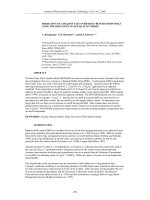
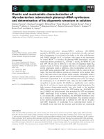
Figure 1 shows the 68 % CL confidence regions for two
parameters of interest, the signal strength relative to the SM
expectation, μ = σ/σSM , and the mass, m H , obtained from
the H → ZZ → 4 and γ γ channels, which have excellent
mass resolution. The combined 68 % CL confidence region,
bounded by a black curve in Fig. 1, is calculated assuming

123

-1

-1

19.7 fb (8 TeV) + 5.1 fb (7 TeV)

σ/σSM

the H → τ τ and H → WW contributions are considered
as signal in the τ τ decay tag analysis. This treatment leads
to an increased sensitivity to the presence of a Higgs boson

that decays into both τ τ and WW.
– The search for invisible Higgs decays of Ref. [28] includes
a modest contribution to the sensitivity from the analysis
targeting ZH production with Z → bb decays. The events
selected by that analysis overlap with those of the analysis
of VH production with H → bb decays, and are therefore
not considered in this combination. Given the limited sensitivity of that search, the overall sensitivity to invisible
decays is not significantly impacted.
– The contribution from the gg → ZH process was not
included in Ref. [21] as calculations for the cross section
as a function of pT (Z) were not available. Since then,
the search for VH production with H → bb has been
augmented by the use of recent NLO calculations for the
gg → ZH contribution [176–179]. In the Z(νν)H(bb) and
Z( )H(bb) channels, the addition of this process leads to
an increase of the expected signal yields by 10 % to 30 %
for pT (Z) around and above 150 GeV. When combined
with the unchanged WH channels, the overall expected
sensitivity for VH production with H → bb increases by
about 10 %.

Eur. Phys. J. C (2015) 75:212

CMS

Combined

2.0 H → γ γ + H → ZZ

H → γ γ tagged

H → ZZ tagged

1.5

1.0

0.5

0.0

123

124

125

126

127

mH (GeV)
Fig. 1 The 68 % CL confidence regions for the signal strength σ/σSM
versus the mass of the boson m H for the H → γ γ and H → ZZ →
4 final states, and their combination. The symbol σ/σSM denotes the
production cross section times the relevant branching fractions, relative
to the SM expectation. In this combination, the relative signal strength
for the two decay modes is set to the expectation for the SM Higgs
boson

the relative event yield between the two channels as predicted

by the SM, while the overall signal strength is left as a free
parameter.
To extract the value of m H in a way that is not completely
dependent on the SM prediction for the production and decay
ratios, the signal strength modifiers for the (ggH, ttH) →
γ γ , (VBF, VH) → γ γ , and pp → H → ZZ → 4 processes are taken as independent, unconstrained, parameters.
The signal in all channels is assumed to be due to a single
state with mass m H . The best-fit value of m H and its uncertainty are extracted from a scan of the combined test statistic q(m H ) with the three signal strength modifiers profiled
together with all other nuisance parameters; i.e. the signal
strength modifiers float freely in the fits performed to scan
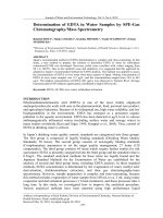
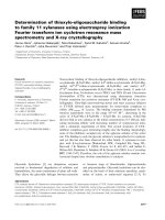
q(m H ). Figure 2 (left) shows the scan of the test statistic
as a function of the mass m H separately for the H → γ γ
and H → ZZ → 4 channels, and for their combination.
The intersections of the q(m H ) curves with the thick horizontal line at 1.00 and thin line at 3.84 define the 68 % and
95 % CL confidence intervals for the mass of the observed
particle, respectively. These intervals include both the statistical and systematic uncertainties. The mass is measured
+0.29
GeV. The less precise evaluations
to be m H = 125.02−0.31
from the H → WW analysis [22], m H = 128+7
−5 GeV, and
from the H → τ τ analysis [23], m H = 122 ± 7 GeV, are
compatible with this result.


Eur. Phys. J. C (2015) 75:212

Page 11 of 50 212

10

H → γ γ tagged
H → ZZ tagged
Combined:
stat. + syst.
stat. only

9 CMS
H → γ γ + H → ZZ
8
μ , μ (ggH,ttH),
γγ
ZZ

μ (VBF,VH)

7

γγ

+0.26

19.7 fb-1 (8 TeV) + 5.1 fb-1 (7 TeV)

- 2 Δ ln L

- 2 Δ ln L

19.7 fb-1 (8 TeV) + 5.1 fb-1 (7 TeV)

+0.14

mH = 125.02- 0.27 (stat)- 0.15 (syst)

10

5

5

4

4

3

3

2

2

1

1
124

125

126

127

mH (GeV)

ZZ

γγ

γγ

μγ γ (VBF,VH), mH

7
6

123

μ , μ (ggH,ttH),

8

6

0

H → γ γ + H → ZZ

9 CMS

0

-2

-1.5

-1

mγHγ

-0.5

-

m4l
H

0

(GeV)

Fig. 2 (Left) Scan of the test statistic q(m H ) = −2 ln L versus the
mass of the boson m H for the H → γ γ and H → ZZ → 4 final
states separately and for their combination. Three independent signal
strengths, (ggH, ttH) → γ γ , (VBF, VH) → γ γ , and pp → H →

ZZ → 4 , are profiled together with all other nuisance parameters.
γγ
(Right) Scan of the test statistic q(m H − m 4H ) versus the difference
between two individual mass measurements for the same model of signal strengths used in the left panel

To evaluate the statistical component of the overall uncertainty, we also perform a scan of q(m H ) fixing all nuisance
parameters to their best-fit values, except those related to
the H → γ γ background models; given that the H → γ γ
background distributions are modelled from fits to data, their
degrees of freedom encode fluctuations which are statistical in nature. The result is shown by the dashed curve in
Fig. 2 (left). The crossings of the dashed curve with the thick
horizontal line define the 68 % CL confidence interval for
+0.26
the statistical uncertainty in the mass measurement: −0.27
GeV. We derive the systematic uncertainty assuming that
the total uncertainty is the sum in quadrature of the statistical and systematic components; the full result is m H =
+0.26
+0.14
(stat) −0.15
(syst) GeV. The median expected
125.02 −0.27
uncertainty is evaluated using an Asimov pseudo-data sample [182] constructed from the best-fit values obtained when
testing for the compatibility of the mass measurement in the
H → γ γ and H → ZZ → 4 channels. The expected uncer+0.26
(stat) ± 0.14 (syst) GeV, in good
tainty thus derived is −0.25
agreement with the observation in data. As a comparison, the
median expected uncertainty is also derived by constructing
an Asimov pseudo-data sample as above except that the signal strength modifiers are set to unity (as expected in the SM)
γγ
and m H = m 4H = 125 GeV, leading to an expected uncertainty of ±0.28 (stat) ± 0.13 (syst) GeV. As could be anticipated, the statistical uncertainty is slightly larger given that
the observed signal strength in the H → γ γ channel is larger
than unity, and the systematic uncertainty is slightly smaller

given the small mass difference between the two channels
that is observed in data.
To quantify the compatibility of the H → γ γ and H →
ZZ mass measurements with each other, we perform a scan of
γγ
the test statistic q(m H −m 4H ), as a function of the difference
between the two mass measurements. Besides the three signal
strength modifiers, there are two additional parameters in this
γγ
test: the mass difference and m H . In the scan, the three signal
γγ
strengths and m H are profiled together with all nuisance
parameters. The result from the scan shown in Fig. 2 (right)
γγ
γγ
+0.56
GeV. From evaluating q(m H −
is m H − m 4H = −0.89−0.57
m 4H = 0) it can be concluded that the mass measurements in
H → γ γ and H → ZZ → 4 agree at the 1.6σ level.
To assess the dependency of the result on the SM Higgs
boson hypothesis, the measurement of the mass is repeated
using the same channels, but with the following two sets of
assumptions: (i) allowing a common signal strength modifier to float, which corresponds to the result in Fig. 1, and
(ii) constraining the relative production cross sections and
branching fractions to the SM predictions, i.e. μ = 1. The
results from these two alternative measurements differ by
less than 0.1 GeV from the main result, both in terms of the
best-fit value and the uncertainties.
4.2 Direct limits on the width of the observed state

For m H ∼ 125 GeV the SM Higgs boson is predicted to be
narrow, with a total width ΓSM ∼ 4 MeV. From the study of

123


212 Page 12 of 50

5 Significance of the observations in data
This section provides an assessment of the significance of
the observed excesses at the best-fit mass value, m H =
125.0 GeV.
Table 2 summarizes the median expected and observed
local significance for a SM Higgs boson mass of 125.0 GeV
from the different decay mode tags, grouped as described
in Sect. 3.3. The value of m H is fixed to the best-fit combined measurement presented in Sect. 4.1. The values of
the expected significance are evaluated using the post-fit
expected background rates and the signal rates expected from
the SM. In the three diboson decay mode tags, the significance is close to, or above, 5σ . In the τ τ decay mode tag the
significance is above 3σ .
Differences between the results in Table 2 and the individual publications are understood in terms of the discussion
in Sects. 3.3 and 3.4, namely the grouping of channels by

123

-1

- 2 Δ ln L

off-shell Higgs boson production, CMS has previously set

an indirect limit on the total width, Γtot /ΓSM < 5.4 (8.0)
observed (expected) at the 95 % CL [27]. While that result
is about two orders of magnitude better than the experimental mass resolution, it relies on assumptions on the underlying theory, such as the absence of contributions to Higgs
boson off-shell production from particles beyond the standard model. In contrast, a direct limit does not rely on such
assumptions and is only limited by the experimental resolution.
The best experimental mass resolution, achieved in the
H → γ γ and H → ZZ → 4 analyses, is typically
between 1 GeV and 3 GeV, as shown in Table 1. The resolution depends on the energy, rapidity, and azimuthal angle
of the decay products, and on the flavour of the leptons in
the case of the H → ZZ → 4 decay. If found inconsistent
with the expected detector resolution, the total width measured in data could suggest the production of a resonance
with a greater intrinsic width or the production of two quasidegenerate states.
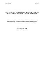
To perform this measurement the signal models in the
H → γ γ and H → ZZ → 4 analyses allow for a natural width using the relativistic Breit–Wigner distribution,
as described in Refs. [16,18]. Figure 3 shows the likelihood
scan as a function of the assumed natural width. The mass of
the boson and a common signal strength are profiled along
with all other nuisance parameters. The dashed lines show the
expected results for the SM Higgs boson. For the H → γ γ
channel the observed (expected) upper limit at the 95 % CL is
2.4 (3.1) GeV. For the H → ZZ → 4 channel the observed
(expected) upper limit at the 95 % CL is 3.4 (2.8) GeV. For
the combination of the two analyses, the observed (expected)
upper limit at the 95 % CL is 1.7 (2.3) GeV.

Eur. Phys. J. C (2015) 75:212
-1

19.7 fb (8 TeV) + 5.1 fb (7 TeV)

10

CMS

9

Combined
Observed
Expected

H → γ γ + H → ZZ
mH, μ

8

H→γ γ tagged
Observed
Expected

7

H→ZZ tagged

6

Observed
Expected

5
4

3
2
1
0

0

2

4

6

Higgs boson width (GeV)
Fig. 3 Likelihood scan as a function of the width of the boson. The
continuous (dashed) lines show the observed (expected) results for the
H → γ γ analysis, the H → ZZ → 4 analysis, and their combination.
The data are consistent with ΓSM ∼ 4 MeV and for the combination of
the two channels the observed (expected) upper limit on the width at
the 95 % CL is 1.7 (2.3) GeV
Table 2 The observed and median expected significances of the
excesses for each decay mode group, assuming m H = 125.0 GeV. The
channels are grouped by decay mode tag as described in Sect. 3.3; when
there is a difference in the channels included with respect to the published results for the individual channels, the result for the grouping
used in those publications is also given
Channel grouping

Significance (σ )
Observed

Expected

H → ZZ tagged

6.5

6.3

H → γ γ tagged

5.6

5.3

H → WW tagged

4.7

5.4

Grouped as in Ref. [22]
H → τ τ tagged
Grouped as in Ref. [23]
H → bb tagged
Grouped as in Ref. [21]
H → μμ tagged

4.3

5.4

3.8

3.9

3.9

3.9

2.0

2.6

2.1

2.5

<0.1

0.4

decay mode tag, the change of the m H value at which the
significance of the H → ZZ → 4 and H → WW analyses
is evaluated, and the treatment of H → WW as part of the
signal, instead of background, in the H → τ τ analysis.
Finally, the observation of the H → γ γ and H → ZZ →
4 decay modes indicates that the new particle is a boson,
and the diphoton decay implies that its spin is different from
unity [190,191]. Other observations, beyond the scope of this

Eur. Phys. J. C (2015) 75:212

paper, disfavour spin-1 and spin-2 hypotheses and, assuming
that the boson has zero spin, are consistent with the pure
scalar hypothesis, while disfavouring the pure pseudoscalar
hypothesis [16,22,41].
6 Compatibility of the observed yields with the SM
Higgs boson hypothesis
The results presented in this section focus on the Higgs boson
production and decay modes, which can be factorized under
the narrow-width approximation, leading to Ni j ∼ σi B j ,
where Ni j represents the event yield for the combination of
production mode i and decay mode j, σi is the production
cross section for production process i, and B j is the branching
fraction into decay mode j. Studies where the production and
decay modes are interpreted in terms of underlying couplings
of particles to the Higgs boson are presented in Sect. 7.
The size of the current data set permits many compatibility tests between the observed excesses and the expected SM
Higgs boson signal. These compatibility tests do not constitute measurements of any physics parameters per se, but
rather allow one to probe for deviations of the various observations from the SM expectations. The tests evaluate the compatibility of the data observed in the different channels with
the expectations for the SM Higgs boson with a mass equal
to the best-fit value found in Sect. 4.1, m H = 125.0 GeV.
This section is organized by increasing degree of complexity of the deviations being probed. In Sect. 6.1 we assess
the compatibility of the overall signal strength for all channels combined with the SM Higgs hypothesis. In Sect. 6.2
the compatibility is assessed by production tag group, decay
tag group, and production and decay tag group. We then
turn to the study of production modes. Using the detailed
information on the expected SM Higgs production contributions, Sect. 6.3 discusses, for each decay tag group, the
results of considering two signal strengths, one scaling the

ggH and ttH contributions, and the other scaling the VBF
and VH contributions. Then, assuming the expected relative
SM Higgs branching fractions, Sect. 6.4 provides a combined
analysis for signal strengths scaling the ggH, VBF, VH, and
ttH contributions individually. Turning to the decay modes,
Sect. 6.5 performs combined analyses of signal strength
ratios between different decay modes, where some uncertainties from theory and some experimental uncertainties cancel
out. Finally, using the structure of the matrix of production
and decay mode signal strengths, Sect. 6.6 tests for the possibility that the observations are due to the presence of more
than one state degenerate in mass.
6.1 Overall signal strength
The best-fit value for the common signal strength modifier
μˆ = σˆ /σSM , obtained from the combined analysis of all

Page 13 of 50 212

channels, provides the simplest compatibility test. In the formal fit, μˆ is allowed to become negative if the observed
number of events is smaller than the expected yield for
the background-only hypothesis. The observed μ,
ˆ assum+0.14
, consistent with unity, the
ing m H = 125.0 GeV, is 1.00−0.13
expectation for the SM Higgs boson. This value is shown as
the vertical bands in the three panels of Fig. 4.
The total uncertainty can be broken down into a statistical component (stat); a component associated with the
uncertainties related to renormalization and factorization
scale variations, parton distribution functions, branching
fractions, and underlying event description (theo); and any
other systematic uncertainties (syst). The result is 1.00 ±
+0.08

(theo) ± 0.07 (syst). Evolution of the SM
0.09 (stat) −0.07
predictions may not only reduce the associated uncertainties
from theory, but also change the central value given above.
6.2 Grouping by predominant decay mode and/or
production tag
One step in going beyond a single signal strength modifier
is to evaluate the signal strength in groups of channels from
different analyses. The groups chosen reflect the different
production tags, predominant decay modes, or both. Once
the fits for each group are performed, a simultaneous fit to all
groups is also performed to assess the compatibility of the
results with the SM Higgs boson hypothesis.
Figure 4 shows the μˆ values obtained in different independent combinations of channels for m H = 125.0 GeV,
grouped by additional tags targeting events from particular production mechanisms, by predominant decay mode, or
both. As discussed in Sect. 3.3, the expected purities of the
different tagged samples vary substantially. Therefore, these
plots cannot be interpreted as compatibility tests for pure
production mechanisms or decay modes, which are studied
in Sect. 6.4.
For each type of grouping, the level of compatibility with
the SM Higgs boson cross section can be quantified by the
value of the test statistic function of the signal strength parameters simultaneously fitted for the N channels considered in
the group, μ1 , μ2 , . . . , μ N ,
qμ = −2 ln L = −2 ln

L(data | μi , θˆμi )
L(data | μˆ i , θˆ )

(5)

evaluated for μ1 = μ2 = · · · = μ N = 1. For each type of
grouping, the corresponding qμ (μ1 = μ2 = · · · = μ N = 1)
from the simultaneous fit of N signal strength parameters is
expected to behave asymptotically as a χ 2 distribution with
N degrees of freedom (dof).
The results for the four independent combinations grouped
by production mode tag are depicted in Fig. 4 (top left). An
excess can be seen for the ttH-tagged combination, due to the

123


212 Page 14 of 50

Eur. Phys. J. C (2015) 75:212

19.7 fb-1 (8 TeV) + 5.1 fb-1 (7 TeV)

CMS

Combined

μ = 1.00 ± 0.14

p

SM

19.7 fb-1 (8 TeV) + 5.1 fb-1 (7 TeV)

mH = 125 GeV

CMS

Combined

μ = 1.00 ± 0.14

= 0.24

p

SM

mH = 125 GeV

= 0.96

H → γ γ tagged

μ = 1.12 ± 0.24

Untagged
μ = 0.87 ± 0.16

H → ZZ tagged

μ = 1.00 ± 0.29

VBF tagged
μ = 1.15 ± 0.27

H → WW tagged
μ = 0.83 ± 0.21

VH tagged

H → ττ tagged

μ = 0.83 ± 0.35

μ = 0.91 ± 0.28

ttH tagged

H → bb tagged

μ = 2.75 ± 0.99

μ = 0.84 ± 0.44

0

1

2

3

4

0

0.5

Best fit σ/σSM

1

1.5

2

Best fit σ/σSM

-1

-1

19.7 fb (8 TeV) + 5.1 fb (7 TeV)
Combined

H → γ γ (untagged) CMS
H → γ γ (VBF tag) pSM = 0.84
H → γ γ (VH tag)
H → γ γ (ttH tag)
H → ZZ (0/1-jet)
H → ZZ (2-jet)
H → WW (0/1-jet)

H → WW (VBF tag)
H → WW (VH tag)
H → WW (ttH tag)
H → ττ (0/1-jet)
H → ττ (VBF tag)
H → ττ (VH tag)
H → ττ (ttH tag)
H → bb (VH tag)
H → bb (ttH tag)
-4
-2

mH = 125 GeV

μ = 1.00 ± 0.14

0

2

4

6

Best fit σ/σSM
Fig. 4 Values of the best-fit σ/σSM for the overall combined analysis
(solid vertical line) and separate combinations grouped by production
mode tag, predominant decay mode, or both. The σ/σSM ratio denotes
the production cross section times the relevant branching fractions, relative to the SM expectation. The vertical band shows the overall σ/σSM
uncertainty. The horizontal bars indicate the ±1 standard deviation

uncertainties in the best-fit σ/σSM values for the individual combinations; these bars include both statistical and systematic uncertainties.

(Top left) Combinations grouped by analysis tags targeting individual
production mechanisms; the excess in the ttH-tagged combination is
largely driven by the ttH-tagged H → γ γ and H → WW channels as
can be seen in the bottom panel. (Top right) Combinations grouped by
predominant decay mode. (Bottom) Combinations grouped by predominant decay mode and additional tags targeting a particular production
mechanism

observations in the ttH-tagged H → γ γ and H → leptons
analyses that can be appreciated from the bottom panel. The
simultaneous fit of the signal strengths for each group of

production process tags results in χ 2 /dof = 5.5/4 and an
asymptotic p-value of 0.24, driven by the excess observed in
the group of analyses tagging the ttH production process.

123


Eur. Phys. J. C (2015) 75:212

Page 15 of 50 212

The results for the five independent combinations grouped
by predominant decay mode are shown in Fig. 4 (top
right). The simultaneous fit of the corresponding five signal
strengths yields χ 2 /dof = 1.0/5 and an asymptotic p-value
of 0.96.
The results for sixteen individual combinations grouped

by production tag and predominant decay mode are shown
in Fig. 4 (bottom). The simultaneous fit of the corresponding
signal strengths gives a χ 2 /dof = 10.5/16, which corresponds to an asymptotic p-value of 0.84.
The p-values above indicate that these different ways of
splitting the overall signal strength into groups related to
the production mode tag, decay mode tag, or both, all yield
results compatible with the SM prediction for the Higgs
boson, μ = μi = 1. The result of the ttH-tagged combination is compatible with the SM hypothesis at the 2.0σ level.

and with the VBF and VH production mechanisms, μggH,ttH
and μVBF,VH , respectively. The five sets of contours correspond to the five predominant decay mode groups, introduced
in Sect. 3.3. It can be seen in Fig. 5 (left) how the analyses
in the H → bb decay group constrain μVBF,VH more than
μggH,ttH , reflecting the larger sensitivity of the analysis of VH
production with H → bb with respect to the analysis of ttH
production with H → bb. An almost complementary situation can be found for the H → ZZ analysis, where the data
constrain μggH,ttH better than μVBF,VH , reflecting the fact
that the analysis is more sensitive to ggH, the most abundant
production mode. The SM Higgs boson expectation of (1, 1)
is within the 68 % CL confidence regions for all predominant
decay groups. The best-fit values for each decay tag group
are given in Table 5.
The ratio of μVBF,VH and μggH,ttH provides a compatibility check with the SM Higgs boson expectation that can
be combined across all decay modes. To perform the measurement of μVBF,VH /μggH,ttH , the SM Higgs boson signal
yields in the different production processes and decay modes
are parameterized according to the scaling factors presented
in Table 4. The fit is performed simultaneously in all channels
of all analyses and takes into account, within each channel,
the full detail of the expected SM Higgs contributions from
the different production processes and decay modes.

Figure 5 (right) shows the likelihood scan of the data for
μVBF,VH /μggH,ttH , while the bottom part of Table 5 shows
the corresponding values; the best-fit μVBF,VH /μggH,ttH is
+0.62
, compatible with the expectation
observed to be 1.25−0.44
for the SM Higgs boson, μVBF,VH /μggH,ttH = 1.

6.3 Fermion- and boson-mediated production processes
and their ratio

6.4 Individual production modes

The four main Higgs boson production mechanisms can
be associated with either couplings of the Higgs boson to
fermions (ggH and ttH) or vector bosons (VBF and VH).
Therefore, a combination of channels associated with a particular decay mode tag, but explicitly targeting different production mechanisms, can be used to test the relative strengths
of the couplings to the vector bosons and fermions, mainly
the top quark, given its importance in ggH production. The
categorization of the different channels into production mode
tags is not pure. Contributions from the different signal processes, evaluated from Monte Carlo simulation and shown in
Table 1, are taken into account in the fits, including theory
and experimental uncertainties; the factors used to scale the
expected contributions from the different production modes
are shown in Table 3 and do not depend on the decay mode.
For a given decay mode, identical deviations of μVBF,VH
and μggH,ttH from unity may also be due to a departure of the
decay partial width from the SM expectation.
Figure 5 (left) shows the 68 % CL confidence regions for
the signal strength modifiers associated with the ggH and ttH

While the production modes can be grouped by the type of
interaction involved in the production of the SM Higgs boson,
as done in Sect. 6.3, the data set and analyses available allow
us to explore signal strength modifiers for different production modes, μggH , μVBF , μVH , and μttH . These scaling factors
are applied to the expected signal contributions from the SM
Higgs boson according to their production mode, as shown in
Table 6. It is assumed that the relative values of the branching
fractions are those expected for the SM Higgs boson. This
assumption is relaxed, in different ways, in Sects. 6.5 and
6.6.
Figure 6 summarizes the results of likelihood scans for the
four parameters of interest described in Table 6 in terms of the
68 % CL (inner) and 95 % CL (outer) confidence intervals.
When scanning the likelihood of the data as a function of one
parameter, the other parameters are profiled.
Table 7 shows the best-fit results for the 7 TeV and 8 TeV
data sets separately, as well as for the full combined analysis. Based on the combined likelihood ratio values for each
parameter, Table 7 also shows the observed significance, the

Table 3 Parameterization used to scale the expected SM Higgs boson
yields from the different production modes when obtaining the results
presented in Table 5 and Fig. 5 (left). The signal strength modifiers
μggH,ttH and μVBF,VH , common to all decay modes, are associated with
the ggH and ttH and with the VBF and VH production mechanisms,
respectively
Parameters of interest: μggH,ttH and μVBF,VH
Signal model H → γ γ H → ZZ H → WW H → τ τ
μggH,ttH

ggH

μggH,ttH

VBF

μVBF,VH μVBF,VH μVBF,VH

μVBF,VH μVBF,VH

VH

μVBF,VH μVBF,VH μVBF,VH

μVBF,VH μVBF,VH

ttH

μggH,ttH

μggH,ttH

μggH,ttH

μggH,ttH

μggH,ttH

μggH,ttH

H → bb
μggH,ttH

μggH,ttH

123


212 Page 16 of 50

Eur. Phys. J. C (2015) 75:212
-1

-1

H → γ γ tagged
H → ZZ tagged
H → WW tagged
H → ττ tagged
H → bb tagged
SM Higgs

CMS

4

19.7 fb (8 TeV) + 5.1 fb-1 (7 TeV)

- 2 Δ ln L

6

μ

VBF,VH

19.7 fb (8 TeV) + 5.1 fb-1 (7 TeV)

10

9 CMS

Observed
Exp. for SM H

8
7
6
5

2

4
3
0

2
1

-1

0

1

2

3

μ

0
0

0.5

1

1.5

2

2.5

μ

ggH,ttH

3

3.5

/μ

VBF,VH

4

ggH,ttH

Fig. 5 (Left) The 68 % CL confidence regions (bounded by the solid
curves) for the signal strength of the ggH and ttH and of the VBF
and VH production mechanisms, μggH,ttH and μVBF,VH , respectively.
The crosses indicate the best-fit values obtained in each group of predominant decay modes: γ γ , ZZ, WW, τ τ , and bb. The diamond at
(1, 1) indicates the expected values for the SM Higgs boson. (Right)
Likelihood scan versus the ratio μVBF,VH /μggH,ttH , combined for all

channels. The fit for μVBF,VH /μggH,ttH is performed while profiling
the five μggH,ttH parameters, one per visible decay mode, as shown in
Table 4. The solid curve represents the observed result in data while the
dashed curve indicates the expected median result in the presence of
the SM Higgs boson. Crossings with the horizontal thick and thin lines
denote the 68 % CL and 95 % CL confidence intervals, respectively

Table 4 Parameterization used to scale the expected SM Higgs boson
yields for the different production processes and decay modes when
obtaining the μVBF,VH /μggH,ttH results presented in Table 5 and
Fig. 5 (right)

Table 5 The best-fit values for the signal strength of the VBF and VH

and of the ggH and ttH production mechanisms, μVBF,VH and μggH,ttH ,
respectively, for m H = 125.0 GeV. The channels are grouped by decay
mode tag as described in Sect. 3.3. The observed and median expected
results for the ratio of μVBF,VH to μggH,ttH together with their uncertainties are also given for the full combination. In the full combination, μVBF,VH /μggH,ttH is determined while profiling the five μggH,ttH
parameters, one per decay mode, as shown in Table 4

Parameter of interest: R = μVBF,VH /μggH,ttH
γγ

ττ
WW
bb
Other parameters: μggH,ttH , μZZ
ggH,ttH , μggH,ttH , μggH,ttH , and μggH,ttH

Signal
model

H → γγ

ggH

μggH,ttH

VBF
VH
ttH

γγ

γγ
R μggH,ttH
γγ
R μggH,ttH
γγ
μggH,ttH

H → ZZ

H → WW H → τ τ

H → bb

μZZ
ggH,ttH

μWW
ggH,ttH

τ
μτggH,ttH

μbb
ggH,ttH

R μZZ
ggH,ttH
R μZZ
ggH,ttH
μZZ

ggH,ttH

R μWW
ggH,ttH
R μWW
ggH,ttH
μWW
ggH,ttH

τ
R μτggH,ttH
τ
R μτggH,ttH
τ
τ
μggH,ttH

R μbb
ggH,ttH
R μbb
ggH,ttH
μbb
ggH,ttH

expected significance, and the pull of the results with respect
to the SM hypothesis. The observed significance is derived
from the observed likelihood ratio for the background-only
hypothesis, μi = 0, in data. The expected significance is
derived from the likelihood ratio for μi = 0 obtained using
the median expected result for the SM Higgs boson. The

pull with respect to the SM hypothesis is derived from the
observed likelihood ratio for μi = 1; by definition, the
expected pull with respect to the SM hypothesis is zero.
+0.19
. After calThe μggH best-fit value is found to be 0.85−0.16
culating the component of the uncertainty that is statistical in

123

Channel grouping

Best fit (μggH,ttH , μVBF,VH )

H → γ γ tagged

(1.07, 1.24)

H → ZZ tagged

(0.88, 1.75)

H → WW tagged

(0.87, 0.66)

H → τ τ tagged

(0.52, 1.21)

H → bb tagged

(0.55, 0.85)

Combined best fit μVBF,VH /μggH,ttH
Observed (expected)
+0.62
+0.49
(1.00−0.35
)
1.25−0.44

nature (stat) and the component related to the theory inputs
(theo), one can subtract them in quadrature from the total
uncertainty and assign the remainder as the systematic uncer+0.11
+0.10
tainty (syst), yielding 0.85 +0.11
−0.09 (stat) −0.08 (theo) −0.09 (syst).
Advances in the calculation of the ggH cross section, e.g.
when considering higher-order effects, may not only reduce


Eur. Phys. J. C (2015) 75:212

Page 17 of 50 212

Table 6 Parameterization used to scale the expected SM Higgs boson
yields of the different production and decay modes when obtaining the
results presented in Fig. 6
Parameters of interest: μggH , μVBF , μVH , and μttH
Signal model H → γ γ

H → ZZ H → WW H → τ τ H → bb

ggH

μggH

μggH

μggH

μggH

μggH

VBF

μVBF

μVBF

μVBF

μVBF

μVBF

VH

μVH

μVH

μVH

μVH

μVH

ttH

μttH

μttH

μttH

μttH

μttH

19.7 fb-1 (8 TeV) + 5.1 fb-1 (7 TeV)

CMS

ggH

= 0.85+0.19
- 0.16

VBF

= 1.16+0.37
- 0.34

μ

= 0.92+0.38
- 0.36

μ
μ

VH

μ

68% CL
95% CL

formed as a function of μVBF (or μVH ), allowing the modifiers associated with the other production processes to float in
the fit together with the nuisance parameters. In data, the best+0.37
+0.38
, while for μVH it is 0.92−0.36
.
fit result for μVBF is 1.16−0.34
For the ttH production mode, the best-fit value for μttH is
+1.08
. The results for VBF, VH, and ttH are
found to be 2.90−0.94

driven by the corresponding tagged categories, while the contribution from ggH is constrained by the 0-jet and untagged
categories.
The results in Table 7 show a clear observation of Higgs
bosons produced through gluon fusion, and evidence for the
production of Higgs bosons through vector boson fusion,
for which both the expected and observed significances are
above the 3σ level. For VH production, the expected significance is 2.9σ and the observed significance is 2.7σ . The
large best-fit value for μttH is compatible with the results
presented and discussed in Sect. 6.2; the data are compatible
with the μttH = 1 hypothesis at the 2.2σ level. Because of
the different parameterizations used, this significance is not
exactly the same as that found in Sect. 6.2 when considering
the combination of ttH-tagged categories.
6.5 Ratios between decay modes

= 2.90+1.08
- 0.94

the uncertainty above, but also shift the central value. The
signal strengths for the VBF and VH production modes are
assessed independently. Individual likelihood scans are per-

Some of the largest uncertainties in SM Higgs predictions
are related to the production cross sections. In an attempt
to evade those uncertainties, it has been proposed [192,193]
to perform measurements of ratios of the signal strengths
in different decay modes, λ yy,x x = β yy /βx x , where βx x =
B(H→xx)/B(H → xx)SM and B denotes a branching fraction. In such βx x ratios, uncertainties related to the production
and decay predictions for the Higgs boson, as well as some
experimental uncertainties, may cancel out. On the other

hand, the uncertainty in a given ratio will reflect the combined statistical uncertainties of both the yy and x x decay
modes.
To probe the different λ yy,x x , the expected signal yields
for the different production and decay modes are scaled by
the factors shown in Table 8. To reduce the dependency of

Table 7 The best-fit results for independent signal strengths scaling
the ggH, VBF, VH, and ttH production processes; the expected and
observed significances with respect to the background-only hypothesis,
μi = 0; and the pull of the observation with respect to the SM hypoth-

esis, μi = 1. The best-fit results are also provided separately for the
7 TeV and 8 TeV data sets, for which the predicted cross sections differ.
These results assume that the relative values of the branching fractions
are those predicted for the SM Higgs boson

ttH

0

1

2

3

4

5

6

Parameter value
Fig. 6 Likelihood scan results for μggH , μVBF , μVH , and μttH . The
inner bars represent the 68 % CL confidence intervals while the outer
bars represent the 95 % CL confidence intervals. When scanning each
individual parameter, the three other parameters are profiled. The SM
values of the relative branching fractions are assumed for the different
decay modes

Parameter

μggH
μVBF

Best-fit result (68 % CL)

Significance (σ )

Pull to SM

7 TeV

8 TeV

Combined

Observed

Expected

(σ )

+0.37
1.03−0.33

+0.19
0.79−0.17

+0.19
0.85−0.16

6.6

7.4

−0.8

3.7

3.3

+0.4

2.7

2.9

−0.2

3.5

1.2

+2.2

+0.99
1.77−0.90

μVH

<0.99

μttH

<2.19

+0.39
1.02−0.36

+0.41
0.96−0.39
3.27+1.20
−1.04

+0.37
1.16−0.34

+0.38
0.92−0.36

+1.08
2.90−0.94

123


212 Page 18 of 50

Eur. Phys. J. C (2015) 75:212

Table 8 Parameterization used to scale the expected SM Higgs boson yields of the different production and decay modes when obtaining the results
presented in Table 9. The μggH,ttH and μVBF,VH parameters are introduced to reduce the dependency of the results on the SM expectation
Parameters of interest: λ yy,x x , λii,x x , λ j j,x x , and λkk,x x
Other parameters: μggH,ttH and μVBF,VH
Signal model

H → xx

H → yy

H → ii

H → jj

H → kk

ggH

μggH,ttH

μggH,ttH λ yy,x x

μggH,ttH λii,x x

μggH,ttH λ j j,x x

μggH,ttH λkk,x x

VBF

μVBF,VH

μVBF,VH λ yy,x x

μVBF,VH λii,x x

μVBF,VH λ j j,x x

μVBF,VH λkk,x x

VH

μVBF,VH

μVBF,VH λ yy,x x

μVBF,VH λii,x x

μVBF,VH λ j j,x x

μVBF,VH λkk,x x

ttH

μggH,ttH

μggH,ttH λ yy,x x

μggH,ttH λii,x x

μggH,ttH λ j j,x x

μggH,ttH λkk,x x

Table 9 The best-fit results and 68 % CL confidence intervals for signal
strength ratios of the decay mode in each column and the decay mode
in each row, as modelled by the parameterization in Table 8. When
the likelihood of the data is scanned as a function of each individual

parameter, the three other parameters in the same row, as well the production cross sections modifiers μggH,ttH and μVBF,VH , are profiled.
Since each row corresponds to an independent fit to data, the relation
λ yy,x x = 1/λx x,yy is only approximately satisfied

Best-fit λcol,row

H → γγ

H → ZZ

H → WW

H → ττ

H → bb

H → γγ

1

+0.27
0.83−0.22

+0.43
0.71−0.25

+0.44
0.63−0.35

H → ZZ

+0.44
1.06−0.31

+0.38
0.92−0.27

1

+0.42
0.86−0.32

+0.61
0.74−0.41

H → WW
H → ττ
H → bb

+0.41
1.21−0.31
+0.75
1.41−0.45
+1.86
1.60−0.70

1
+0.44
1.10−0.33
+0.81
1.31−0.48
1.48+1.85
−0.70

the results on the expected structure of the SM Higgs production cross section, the μggH,ttH and μVBF,VH parameters
are introduced and allowed to float independently. Therefore,
these measurements only assume the SM ratio of ggH and ttH
cross sections and the ratio of VBF and VH cross sections.
Given the five decay modes that are currently accessible,
four ratios can be probed at a time. For example, the choice of
the H → γ γ decay as denominator, x x = γ γ , fixes the four

ratio parameters to be λZZ,γ γ , λbb,γ γ , λWW,γ γ , and λτ τ,γ γ .
When scanning the likelihood for the data as a function of
a given λ yy,x x ratio, the production cross section modifiers
μggH,ttH and μVBF,VH , as well as the other three ratios, are
profiled. The best-fit results for each choice of denominator
are presented as the different rows in Table 9. While correlated uncertainties from theory and correlated experimental
uncertainties may cancel out to some extent in these ratios,
each ratio includes the statistical uncertainties from the two
decay modes involved. For the available data set and analyses,
the resulting statistical uncertainty dominates the total uncertainty. It can be seen that the SM expectation, λ yy,x x = 1, is
inside the 68 % CL confidence interval for all measurements.
6.6 Search for mass-degenerate states with different
coupling structures
One assumption that is made in Sect. 7 when studying the
couplings of the Higgs boson is that the observations are
due to the manifestation of a single particle. Alternatively, a

123

+0.38
0.88−0.26
+0.68
1.15−0.44

+1.57
1.32−0.59

+0.43
0.76−0.30

1
+1.34
1.14−0.52

+0.59
0.65−0.37
+0.69
0.87−0.49

1

superposition of states with indistinguishable mass values is
expected in models or theories beyond the SM [194–197]. In
this section we explore the validity of this assumption.
Taking advantage of the very good mass resolution in the
H → γ γ analysis, the presence of near mass-degenerate
states has been previously probed down to mass differences
between 2.5 GeV and 4 GeV without evidence for the presence of a second state [18]. Given the finite mass resolution, such searches are not sensitive to a mixture of states
with mass values closer than the resolution itself, such that
other reported measurements would integrate the contributions from both states.
In the case of two or more states with masses closer to each
other than the experimental resolution, it becomes impossible to discern them using the mass observables. However, the
distinction between states can still be made, provided that the
states have different coupling structures, i.e. different coupling strengths to the SM particles. Using the measurements
of the different production and decay tags, as well as the
detailed knowledge of their expected composition in terms
of production processes and decay modes, it is possible to test
the compatibility of the observations with the expectations
from a single state. Several authors discussed this possibility, proposing methods to look for deviations assuming that,
in the presence of more than one state, the individual states

would couple differently to the SM particles [198,199].
A general parameterization of the 5 × 4 matrix, M, of
signal strengths for the different production processes and


Eur. Phys. J. C (2015) 75:212

Page 19 of 50 212

Table 10 A completely general signal parameterization used to scale
the expected yields of the 5 × 4 different production and decay modes.
The particular choice of parameters is such that the single-particle
parameterization shown in Table 11 is a nested model, i.e. it can be

j

obtained by assuming λi = λi , where i runs through the production
processes except ggH and j runs through the decay modes. The expecj
tation for the SM Higgs boson is λi = μ j = 1. This parameterization
is used in the denominator of the test statistic defined in Eq. (6)

All parameters constrained to be positive
Signal model

H → γγ

H → ZZ

H → WW

H → ττ

H → bb

ggH

μγ γ

μZZ

μWW

μτ τ

μbb

λZZ
VBF μZZ
λZZ
VH μZZ
λZZ
ttH μZZ

λWW
VBF
λWW
VH
λWW
ttH

τ μ
λτVBF
ττ
τ
τ μ
λVH
ττ
τ μ
λτttH
ττ

λbb
VBF μbb

VBF
VH
ttH

γγ
λVBF μγ γ
γγ
λVH μγ γ
γγ
λttH μγ γ

Table 11 A general single-state parameterization used to scale the
expected yields of the different production and decay modes. For this
parameterization the matrix has rank(M) = 1 by definition. It can be
seen that this parameterization is nested in the general one presented in
j

Table 10, and can be obtained by setting λi = λi , where i runs through

μWW
μWW
μWW

λbb
VH μbb
λbb
ttH μbb

the production processes except ggH and j runs through the decay
modes. The expectation for the SM Higgs boson is λi = μ j = 1. This
parameterization is used in the numerator of the test statistic defined in
Eq. (6)

All parameters constrained to be positive
Signal model

H → γγ

H → ZZ

H → WW

H → ττ

H → bb

ggH

μγ γ

μZZ

μWW

μτ τ

μbb

VBF

λVBF μγ γ

λVBF μZZ

λVBF μWW

λVBF μτ τ

λVBF μbb

VH

λVH μγ γ

λVH μZZ

λVH μWW

λVH μτ τ

λVH μbb

ttH

λttH μγ γ

λttH μZZ

λttH μWW

λttH μτ τ

λttH μbb

decay modes is shown in Table 10. This parameterization
has as many degrees of freedom as there are elements in
the matrix and is completely general. Depending on whether
there is one particle or more particles responsible for the
observations in data, the algebraic properties of M, namely
its rank, rank(M), will vary.
If there is only one state it follows that rank(M) = 1,
i.e. there should be one common multiplier per row and
one common multiplier per column. A general matrix with
rank(M) = 1 can be parameterized as shown in Table 11.
This parameterization can also be obtained by taking the
most general 5 × 4 parameterization in Table 10 and assumj
ing λi = λi , where i runs through the production processes except ggH and j runs through the decay modes.

Given this relationship, the model for a general matrix with
rank(M) = 1 presented in Table 11 is nested, in the statistics sense, in the general parameterization of the 5 × 4 matrix
presented in Table 10.
The expectation for the SM Higgs boson is a particular
case of a rank 1 matrix, namely that for which λi = μ j = 1,
where i runs through the production processes except ggH
and j runs through the decay modes.
If there is more than one particle contributing to the observations, the structure of M may be such that rank(M) > 1
as a consequence of the different interaction strengths of the
individual, yet mass-degenerate, states.

The procedure to test for the presence of mass-degenerate
states proposed in Ref. [200] takes into account both the fact
that there may be missing matrix elements and the fact that
there are uncertainties in the measurements, including their
correlations. A profile likelihood ratio test statistic, qλ , is built
using two different models for the structure of M, namely
those presented in Tables 10 and 11,
L(data | λi = λˆ i , μˆ j )
.
j
L(data | λˆ , μˆ j )
j

qλ = −2 ln

(6)

i

The test statistic qλ is a function of the 20 variables defined
j
in Table 10: λi and μ j , where the index i runs through the
VBF, VH, and ttH production processes and the index j runs
through the decay modes. In this likelihood ratio, the model
in Table 10 is taken as the alternative hypothesis and corresponds to the so-called “saturated model” in statistics, as it
contains as many degrees of freedom as there are elements
in M. The null hypothesis model is the one presented in
Table 11, which parameterizes M as a general rank 1 matrix,
where all rows are multiples of each other, as expected for a
single particle. If the observations are due to a single particle,
the λi do not depend on the decay mode and the value of the qλ
is not very large, since both hypotheses fit the data equally
well. However, for a matrix with rank(M) = 1, the most

123


Probability density

212 Page 20 of 50

Eur. Phys. J. C (2015) 75:212

19.7 fb-1 (8 TeV) + 5.1 fb-1 (7 TeV)

0.1

CMS

0.09

7 Compatibility of the observed data with the SM Higgs
boson couplings

Observed
Exp. for SM H

0.08
0.07
0.06
0.05
0.04
0.03
0.02
0.01
0

0

5

10

15

20

25

30

35

40

45

q

λ

Fig. 7 Distribution of the profile likelihood ratio qλ between different
assumptions for the structure of the matrix of signal strengths for the
production processes and decay modes both for pseudo-data samples
generated under the SM hypothesis and the value observed in data.
The likelihood in the numerator is that for the data under a model of a
general rank 1 matrix, expected if the observations are due to a single
particle and of which the SM is a particular case. The likelihood in
the denominator is that for the data under a “saturated model” with as
many parameters as there are matrix elements. The arrow represents the
observed value in data, qλobs . Under the SM hypothesis, the probability
to find a value of qλ ≥ qλobs is (7.9 ± 0.3) %, where the uncertainty
reflects only the finite number of pseudo-data samples generated

general 5 × 4 matrix model will fit the data better than the
general rank 1 matrix model and the value of qλ is expected
to be large.
The compatibility of the value of the test statistic observed
in data, qλobs , with the expectation from the SM is evaluated using pseudo-data samples randomly generated under

the SM hypothesis. Figure 7 shows the distribution of qλ for
the SM pseudo-data samples as well as the value observed
in data, qλobs = 12.2. Under the SM hypothesis, we find
that the probability of observing a value of qλ ≥ qλobs is
(7.9 ± 0.3) %, where the uncertainty reflects only the finite
number of pseudo-data samples generated. Such a p-value
corresponds to a deviation from the SM expectation of about
1.4σ . This small tension, not present in previous tests performed in this section, is due to the observed data in the
dijet-tagged channel of the H → ZZ analysis; performing
a fit to a model where the VBF and VH production modes
are floated separately shows that the data prefer a very large
VH contribution and a very small VBF contribution. When
H → ZZ analysis inputs are not considered, the p-value is
found to be about 33 %.

123

Whereas in Sect. 6 the production and decay of the boson
were explored separately, the studies presented in this section
simultaneously investigate the couplings of the boson to SM
particles in the production and decay processes. In this way,
correlations are handled consistently between the production
modes and the decay modes. For example, the coupling of
the SM Higgs boson to the Z boson is involved both in the
ZH production mode and the H → ZZ decay mode, such
that more information can be extracted from a simultaneous
modelling of the production and decay modes in terms of the
couplings involved.
Following the framework laid out in Ref. [171], we assume
the signal arises from a single particle with J PC = 0++ and

a width such that the narrow-width approximation holds, permitting its production and decay to be considered independently. These assumptions are supported by the results of
Sect. 6.6 on the presence of more particles at the same mass,
those of Refs. [40,41] regarding alternative J P assignments
and mixtures, and those of Ref. [27] concerning the width of
the particle.
Under the assumptions above, the event yield in a given
(production)×(decay) mode is related to the production cross
section and the partial and total Higgs boson decay widths
via
(σ B) (x → H → yy) =

σx Γyy
,
Γtot

(7)

where σx is the production cross section through process x,
which includes ggH, VBF, WH, ZH, and ttH; Γyy is the partial
decay width into the final state yy, such as WW, ZZ, bb, τ τ ,
gg, or γ γ ; and Γtot is the total width of the boson.
Some quantities, such as σggH , Γgg , and Γγ γ , are generated by loop diagrams and, therefore, are sensitive to the
presence of certain particles beyond the standard model
(BSM). The possibility of Higgs boson decays to BSM
particles, with a partial width ΓBSM , can also be accommodated by considering Γtot as a dependent parameter so
Γyy + ΓBSM , where
Γyy stands for the
that Γtot =
sum over partial widths for all decays to SM particles.
With the data from the H(inv) searches, ΓBSM can be further broken down as ΓBSM = Γinv + Γundet , where Γinv

can be constrained by searches for invisible decays of the
Higgs boson and Γundet corresponds to Higgs boson decays
not fitting into the previous definitions. The definition of
Γundet is such that two classes of decays can give rise to
Γundet > 0: (i) BSM decays not studied in the analyses used
in this paper, such as hypothetical lepton flavour violating
decays, e.g. H → μτ , and (ii) decays that might not be
detectable with the existing experimental setup because of
the trigger conditions of the experiment, such as hypotheti-


Eur. Phys. J. C (2015) 75:212

cal decays resulting in a large multiplicity of low- pT particles.
To test the observed data for possible deviations from the
rates expected for the SM Higgs boson in the different channels, we introduce coupling modifiers, denoted by the scale
factors κi [171]. The scale factors are defined for production processes by κi2 = σi /σiSM , for decay processes by
κi2 = Γii /ΓiiSM , and for the total width by κH2 = Γtot /ΓSM ,
where the SM values are tabulated in Ref. [171]. When considering the different κi , the index i can represent many ways
to test for deviations:
– For SM particles with tree-level couplings to the Higgs
boson: κW (W bosons), κZ (Z bosons), κb (bottom
quarks), κτ (tau leptons), κt (top quarks), and κμ (muons).
Unless otherwise noted, the scaling factors for other
fermions are tied to those that can be constrained by data.
– Particular symmetries of the SM make it interesting to
test for deviations in whole classes of particles, leading to
κV (massive vector bosons), κf (fermions), κ (leptons),
κq (quarks), κu (up-type fermions), and κd (down-type
fermions).

– For SM particles with loop-induced couplings, the scaling factors can be expressed in terms of the tree-level
coupling modifiers, assuming the SM loop structure, but
can also be taken as effective coupling modifiers: κg (gluons) and κγ (photons).
– The scaling factors for couplings to second generation
fermions are equal to those for the third generation: κs =
κb , κμ = κτ , and κc = κt , except in Sect. 7.4, where κμ
is constrained from the analysis of H → μμ decays.
Given their small expected contributions, the couplings to
electrons, up quarks, and down quarks, are neglected.
In addition to the κi parameters, the existence of BSM
decays, invisible decays, and undetectable decays of the
Higgs boson is considered; the corresponding branching
fractions are denoted BRBSM , BRinv , and BRundet , as in
Ref. [171].
Significant deviations of any κ parameter from unity or
of any BR parameter from zero would imply new physics
beyond the SM Higgs boson hypothesis. The size of the
current data set is insufficient to precisely quantify all phenomenological parameters defining the Higgs boson production and decay rates. Therefore, we present a set of combined analyses of different numbers of parameters, where the
remaining parameters are either set to the SM expectations
or profiled in the likelihood scans together with all other nuisance parameters. The value of m H is fixed to the measured
value of 125.0 GeV, as determined in Sect. 4.1. Since results
for the individual channels are based on different assumed
values of the mass, differences should be expected when com-

Page 21 of 50 212

paring the previously published results from the individual
channels with those in this combined analysis.
This section is organized as follows. In Sect. 7.1 we
explore whether κW and κZ are compatible with each other

and can be meaningfully used together as κV . In Sect. 7.2
we test for deviations that would affect the couplings of
massive vector bosons and fermions differently. The scaling factors among different types of fermions, leptons versus quarks and up-type versus down-type, are investigated in
Sect. 7.3. In Sect. 7.4, we consider the results of a fit for the
tree-level coupling scaling factors and the relation between
the observations and the corresponding particle masses. We
then turn to the study of models where BSM physics could
manifest itself in loops (κg , κγ ) or decays (BRBSM , BRinv ,
BRundet ). In Sect. 7.5 the tree-level couplings are constrained
to those expected in the SM, and the searches for H(inv) are
included. This restriction is lifted in Sect. 7.6, where a coupling scaling factor for the massive vector bosons and individual fermion coupling scaling factors are allowed to float,
while in Sect. 7.7 the total width scaling factor is also left
free to float. In Sect. 7.8, the results from the searches for
invisible decays are included, and from the combination of
the visible and invisible decays, limits on BRundet are set.
Table 12 summarizes the results of the tests performed.
7.1 Relation between the coupling to the W and Z bosons
In the SM, the Higgs sector possesses an approximate
SU(2)L × SU(2)R global symmetry, which is broken by the
Higgs vacuum expectation value to the diagonal subgroup
SU(2)L+R . As a result, the tree-level ratios of the W and Z
boson masses, m W /m Z , and the ratio of their couplings to
the Higgs boson, gW /gZ , are protected against large radiative corrections, a property known as “custodial symmetry” [201,202]. However, large violations of custodial symmetry are possible in new physics models. We focus on the
two scaling factors κW and κZ that modify the couplings of
the SM Higgs boson to the W and Z bosons and perform two
different combined analyses to assess the consistency of the
ratio λWZ = κW /κZ with unity.
The dominant production mechanism populating the 0-jet
and 1-jet channels of the H → WW → ν ν analysis and
the untagged channels of the H → ZZ → 4 analysis is

ggH. Therefore, the ratio of event yields in these channels
provides a nearly model-independent measurement of λWZ .
We perform a combined analysis of these two channels with
two free parameters, κZ and λWZ . The likelihood scan versus
λWZ is shown in Fig. 8 (left). The scale factor κZ is treated
+0.22
, i.e.
as a nuisance parameter. The result is λWZ = 0.94−0.18
the data are consistent with the SM expectation (λWZ = 1).
We also extract λWZ from the combined analysis of all
channels. In this approach, we introduce three parameters:
λWZ , κZ , and κf . The BSM Higgs boson width ΓBSM is set to

123


212 Page 22 of 50

Eur. Phys. J. C (2015) 75:212

Table 12 Tests of the compatibility of the data with the SM Higgs boson
couplings. The best-fit values and 68 % and 95 % CL confidence intervals are given for the evaluated scaling factors κi or ratios λi j = κi /κ j .
Model parameters

Table in Ref. [171]

Parameter

The different compatibility tests discussed in the text are separated by
horizontal lines. When one of the parameters in a group is evaluated,

others are treated as nuisance parameters
Best-fit result

Comment

68 % CL

95 % CL

κZ , λWZ (κf = 1)

–

λWZ

+0.22
0.94−0.18

[0.61, 1.45]

λWZ = κW /κZ from ZZ and 0/1-jet
WW channels

κZ , λWZ , κf

44 (top)

λWZ

+0.14

0.92−0.12

[0.71, 1.24]

λWZ = κW /κZ from full combination

κV

[0.87, 1.14]

κV scales couplings to W and Z bosons

κf

+0.07
1.01−0.07
+0.14
0.87−0.13

[0.63, 1.15]

κf scales couplings to all fermions

κ V , κf

43 (top)

κV , λdu , κu

46 (top)

λdu

+0.19
0.99−0.18

[0.65, 1.39]

λdu = κu /κd , relates up-type and
down-type fermions

κV , λ q , κq

47 (top)

λ

+0.23
1.03−0.21

[0.62, 1.50]

λ

κ W , κZ , κ t , κ b , κ τ , κ μ

Extends 51

κW

+0.14
0.95 −0.13

[0.68, 1.23]

q

+0.16
1.05 −0.16

[0.72, 1.35]

κt

0.81

[0.53, 1.20]

κb

0.74

κτ

0.84

κμ

0.49

M ( GeV)

κZ

+0.19
−0.15
+0.33
−0.29
+0.19
−0.18
+1.38
−0.49

q = κ /κq , relates leptons and
quarks

Up-type quarks (via t)

[0.09, 1.44]

Down-type quarks (via b)

[0.50, 1.24]

κτ scales the coupling to tau leptons

[0.00, 2.77]

κμ scales the coupling to muons

245 ± 15

[217, 279]

V
κf = v M 1+f and κV = v M 1+2

+0.041
0.014−0.036

[−0.054, 0.100]

κg

+0.11
0.89−0.10

[0.69, 1.11]

κγ

+0.12
1.14−0.13

[0.89, 1.40]

48 (middle)

BRBSM

≤ 0.14

[0.00, 0.32]

Allows for BSM decays

With H(inv) searches

–

BRinv

+0.15
0.03 −0.03

[0.00, 0.32]

H(inv) use implies BRundet =0

With H(inv) and κi = 1

–

BRinv

+0.11
0.06 −0.06

[0.00, 0.27]

Assumes κi = 1 and uses H(inv)

50 (bottom)

κgZ

+0.14
0.98 −0.13

M,

Ref. [206]

m

m2

(Sect. 7.4)

κ g , κγ

κg , κγ , BRBSM

κgZ , λWZ , λZg , λbZ , λγ Z , λτ Z , λtg

48 (top)

[0.73, 1.27]

κgZ = κg κZ /κH , i.e. floating κH

+0.15
0.87 −0.13

[0.63, 1.19]

λWZ = κW /κZ

λZg

1.39

[0.87, 2.18]

λZg = κZ /κg

λbZ

0.59

≤1.07

λbZ = κb /κZ

λγ Z

0.93

[0.67, 1.31]

λγ Z = κγ /κZ

λτ Z

0.79

[0.47, 1.20]

λτ Z = κτ /κZ

λtg

2.18

[1.30, 3.35]

λtg = κt /κg

λWZ

123

Effective couplings to gluons (g) and
photons (γ )

+0.36
−0.28
+0.22
−0.23
+0.17

−0.14
+0.19
−0.17
+0.54
−0.46


Eur. Phys. J. C (2015) 75:212

Page 23 of 50 212

Table 12 continued
Model parameters

Table in Ref. [171] Parameter Best-fit result

κ V , κb , κ τ , κ t , κ g , κγ

Similar to 50 (top)

κV

Comment

68 % CL

95 % CL

+0.14
0.96−0.15

[0.66, 1.23]
[0.00, 1.23] Down-type quarks (via b)

κγ

+0.28
0.64−0.29
+0.18
0.82−0.18
+0.34
1.60−0.32
+0.15
0.75−0.13
+0.17
0.98−0.16

[0.00, 0.57] Allows for BSM decays

κb
κτ
κt
κg

[0.48, 1.20] Charged leptons (via τ )
[0.97, 2.28] Up-type quarks (via t)
[0.52, 1.07]
[0.67, 1.33]

With κV ≤ 1 and BRBSM

–

BRBSM

≤0.34

With κV ≤ 1 and H(inv)

–

BRinv

0.17 ± 0.17 [0.00, 0.49] H(inv) use implies BRundet = 0

With κV ≤ 1, H(inv), BRinv , and BRundet –

BRinv

0.17 ± 0.17 [0.00, 0.49] Separates BRinv from BRundet ,
BRBSM = BRinv + BRundet

BRundet

≤0.23

–

-1

-1

CMS

9

Observed

H → VV (0/1 jet)
κ f =1, κ Z, λWZ

8

- 2 Δ ln L

- 2 Δ ln L

-1

19.7 fb (8 TeV) + 5.1 fb (7 TeV)

10

[0.00, 0.52]

Exp. for SM H

CMS

9

8
7

6

6

5

5

4

4

3

3

2

2

1

1
0

0.5

1

1.5

2

λWZ (κf = 1)

0

Observed

κ f , κ Z, λWZ

7

0

-1

19.7 fb (8 TeV) + 5.1 fb (7 TeV)

10

0

0.5

Exp. for SM H

1

1.5

2

λWZ

Fig. 8 Likelihood scans versus λWZ , the ratio of the coupling scaling
factors to W and Z bosons: (left) from untagged pp → H → WW and
pp → H → ZZ searches, assuming the SM couplings to fermions,
κf = 1; (right) from the combination of all channels, profiling the cou-

pling to fermions. The solid curve represents the observation in data.
The dashed curve indicates the expected median result in the presence
of the SM Higgs boson. Crossings with the horizontal thick and thin
lines denote the 68 % CL and 95 % CL confidence intervals, respectively

zero. The partial width Γgg , induced by top and bottom quark
loops, scales as κf2 . The partial width Γγ γ is induced via loop
diagrams, with the W boson and top quark being the dominant
contributors, and is scaled with κγ2 (κb , κτ , κt , κW ), a function
defined in Eq. (113) of Ref. [171]. In the likelihood scan as
a function of λWZ , both κZ and κf are profiled together with
all other nuisance parameters. The introduction of κf carries
with it the assumption that the coupling to all fermions is
common, but possibly different from the SM expectation. The

likelihood scan is shown in Fig. 8 (right) with a solid curve.
The dashed curve indicates the median expected result for the

SM Higgs boson, given the current data set. The measured
value from the combined analysis of all channels is λWZ =
+0.14
and is consistent with the expectation from the SM.
0.92−0.12
Given these results, and unless otherwise noted, in all subsequent measurements we assume λWZ = 1 and use a common factor κV to modify the couplings to W and Z bosons,
while preserving their ratio.

123


212 Page 24 of 50

Eur. Phys. J. C (2015) 75:212

1.5

-1

-1

19.7 fb (8 TeV) + 5.1 fb (7 TeV)

κf

κf

-1

2.0

CMS

2.0

1.8 CMS
1.6

1.0

1.4

0.5

1.2

0.0

1.0

-0.5

0.8

-1.0
-1.5
-2.0
0.0

-1

19.7 fb (8 TeV) + 5.1 fb (7 TeV)

Observed
68% CL
95% CL
99.7% CL
SM Higgs

0.5

0.6
0.4
0.2
1.0

1.5

κV

0.0
0.0

Observed
68% CL
95% CL
99.7% CL
SM Higgs

0.5

1.0

1.5

κV

Fig. 9 Results of 2D likelihood scans for the κV and κf parameters. The
cross indicates the best-fit values. The solid, dashed, and dotted contours
show the 68 %, 95 %, and 99.7 % CL confidence regions, respectively.

The diamond shows the SM point (κV , κf ) = (1, 1). The left plot shows
the likelihood scan in two quadrants, (+, +) and (+, −). The right plot
shows the likelihood scan constrained to the (+, +) quadrant

7.2 Test of the couplings to massive vector bosons
and fermions

In Fig. 9 the 68 %, 95 %, and 99.7 % CL confidence
regions for κV and κf are shown with solid, dashed, and
dotted curves, respectively. The data are compatible with
the expectation for the standard model Higgs boson: the
point (κV , κf ) = (1, 1) is within the 68 % CL confidence
region defined by the data. Because of the way these compatibility tests are constructed, any significant deviations
from (1, 1) would not have a straightforward interpretation
within the SM and would imply BSM physics; the scale and
sign of the best-fit values in the case of significant deviations would guide us in identifying the most plausible BSM
scenarios.
Figure 10 shows the results of this combined analysis in
the different decay mode groups. The role and interplay of

different channels is important. For example, Fig. 9 (left)
shows a region in the (+, −) quadrant, where κV and κf have
opposite signs, which is excluded at the 95 % CL but not at the
99.7 % CL; it can be seen in Fig. 10 (left) how the combined
exclusion in the (+, −) quadrant is foremost due to the ability
of the H → γ γ decay to discern the relative sign between κV
and κf . This is due to the destructive interference between the
amplitudes of the W loops and top quark loops in the H →
γ γ decay: κγ2 ∼ 1.59 κV2 −0.66 κV κf +0.07 κf2 ; if κV and κf
have opposite signs, the interference becomes constructive,
leading to a larger H → γ γ branching fraction. The shapes
of the confidence regions for other decay channels are also
interesting: the analyses of decays to massive vector bosons
constrain κV better than κf , whereas the analyses of decays
to fermions constrain κf better than κV . In the model used
for this analysis, the total width scales as κH2 ∼ 0.75 κf2 +

In the SM, the nature of the coupling of the Higgs boson
to fermions, through a Yukawa interaction, is different from
the nature of the Higgs boson coupling to the massive vector
bosons, a result of electroweak symmetry breaking. Some
BSM models predict couplings to fermions and massive vector bosons different from those in the SM.
We compare the observations in data with the expectation
for the SM Higgs boson by fitting two parameters, κV and
κf , where κV = κW = κZ is a common scaling factor for
massive vector bosons, and κf = κb = κt = κτ is a common scaling factor for fermions. We assume that ΓBSM = 0.
At leading order, all partial widths scale either as κV2 or κf2 ,
except for Γγ γ . As discussed in Sect. 7.1, the partial width
Γγ γ is induced via loops with virtual W bosons or top quarks
and scales as a function of both κV and κf . For that reason,

the H → γ γ channel is the only channel being combined
that is sensitive to the relative sign of κV and κf .
Figure 9 shows the 2D likelihood scan over the (κV , κf )
parameter space. While Fig. 9 (left) allows for different signs
of κV and κf , Fig. 9 (right) constrains the scan to the (+, +)
quadrant that contains the SM expectation (1, 1). The (−, −)
and (−, +) quadrants are not shown since they are degenerate
with respect to the ones studied, with the implication that
with the available analyses we can only probe whether κV
and κf have the same sign or different signs. Studies of the
production of a Higgs boson associated with a single top
quark can, in principle, lift that degeneracy.

123


Eur. Phys. J. C (2015) 75:212
19.7 fb-1 (8 TeV) + 5.1 fb-1 (7 TeV)
H→WW

1
H→ZZ

%
95

L.

C.

H→ττ

19.7 fb-1 (8 TeV) + 5.1 fb-1 (7 TeV)

Observed
SM Higgs

κf

H→
γγ

κf

Observed
SM Higgs

CMS

2

H→WW

H→γ γ

CMS

2

Page 25 of 50 212

1.5

H→bb

1

-1

0.5

H→ττ
95
%

C.L
.

0

-2

0

0.5

1

1.5

κV

0

H→ZZ

0

0.5

1

H→bb

κV

1.5

Fig. 10 The 68 % CL confidence regions for individual channels
(coloured swaths) and for the overall combination (thick curve) for the
κV and κf parameters. The cross indicates the global best-fit values. The
dashed contour bounds the 95 % CL confidence region for the combi-

nation. The diamond represents the SM expectation, (κV , κf ) = (1, 1).
The left plot shows the likelihood scan in two quadrants (+, +) and
(+, −), the right plot shows the positive quadrant only

0.25 κV2 , reflecting the large expected contributions from the
bottom quark and W boson.
The 95 % CL confidence intervals for κV and κf , obtained

from a scan where the other parameter is floated, are
[0.87, 1.14] and [0.63, 1.15], respectively.

positive, the 95 % CL confidence intervals are found to be
[0.65, 1.39] and [0.62, 1.50], respectively. There is no evidence that different classes of fermions have different scaling
factors.

7.3 Test for asymmetries in the couplings to fermions

7.4 Test of the scaling of couplings with the masses of SM
particles

In models with two Higgs doublets (2HDM) [203], the couplings of the neutral Higgs bosons to fermions can be substantially modified with respect to the couplings predicted for
the SM Higgs boson. For example, in the minimal supersymmetric standard model [204], the couplings of neutral Higgs
bosons to up-type and down-type fermions are modified, with
the modification being the same for all three generations and
for quarks and leptons. In more general 2HDMs, leptons can
be made to virtually decouple from one Higgs boson that
otherwise behaves in a SM-like way with respect to the W
bosons, Z bosons, and quarks. Inspired by the possibility
of such modifications to the fermion couplings, we perform
two combinations in which we allow for different ratios of
the couplings to down-type fermions and up-type fermions
(λdu = κd /κu ) or different ratios of the couplings to leptons
and quarks (λ q = κ /κq ).
Figure 11 (left) shows the likelihood scan versus λdu , with
κV and κu profiled together with all other nuisance parameters. Figure 11 (right) shows the likelihood scan versus λ q ,
with κV and κq profiled. Assuming that both λdu and λ q are

Under the assumption that there are no interactions of the

Higgs boson other than to the massive SM particles, the data
allow a fit for deviations in κW , κZ , κb , κτ , κt , and κμ . In
this fit, the loop-induced processes (σggH , Γgg , and Γγ γ ) are
expressed in terms of the above tree-level κ parameters and
are scaled according to their SM loop structure. The result for
this fit is displayed in Fig. 12 (left) and shows no significant
deviations from the SM expectation. The small uncertainty
in the κt parameter directly reflects the fact that in this model,
the ggH production mode is being described in terms of κt
and κb , κg2 ∼ 1.11 κt2 + 0.01 κt κb − 0.12 κb2 , such that κb
has a small contribution.
In the SM, the Yukawa coupling between the Higgs boson
and the fermions, λf , is proportional to the mass of the
fermion, m f . This is in contrast with the coupling to weak
bosons, gV , which involves the square of the mass of the weak
boson, m V . With these differences in mind, it is possible to
motivate a phenomenological parameterization relating the
masses of the fermions and weak bosons to the corresponding κ modifiers using two parameters, M and [205,206].

123