(SPE78168MS) New Model for Predicting the Rate of Sand Production
Bạn đang xem bản rút gọn của tài liệu. Xem và tải ngay bản đầy đủ của tài liệu tại đây (387.03 KB, 9 trang )
SPE/ISRM 78168
New Model for Predicting the Rate of Sand Production
S.M. Willson (BP America Inc.), Z.A. Moschovidis, J.R. Cameron (PCM Technical Inc.) & I.D. Palmer (BP America Inc.)
Copyright 2002, Society of Petroleum Engineers Inc.
This paper was prepared for presentation at the SPE/ISRM Rock Mechanics Conference held
in Irving, Texas, 20-23 October 2002.
This paper was selected for presentation by an SPE/ISRM Program Committee following
review of information contained in an abstract submitted by the author(s). Contents of the
paper, as presented, have not been reviewed by the Society of Petroleum Engineers or
International Society of Rock Mechanics and are subject to correction by the author(s). The
material, as presented, does not necessarily reflect any position of the Society of Petroleum
Engineers, International Society of Rock Mechanics, its officers, or members. Papers
presented at SPE/ISRM meetings are subject to publication review by Editorial Committees of
the Society of Petroleum Engineers. Electronic reproduction, distribution, or storage of any part
of this paper for commercial purposes without the written consent of the Society of Petroleum
Engineers is prohibited. Permission to reproduce in print is restricted to an abstract of not more
than 300 words; illustrations may not be copied. The abstract must contain conspicuous
acknowledgment of where and by whom the paper was presented. Write Librarian, SPE, P.O.
Box 833836, Richardson, TX 75083-3836, U.S.A., fax 01-972-952-9435.
Abstract
A number of robust predictive methods for establishing
sanding thresholds have been developed over the past decade.
Having identified when the onset of sanding occurs, recent
research efforts have focused on determining the rate at which
sand will be produced once these thresholds are exceeded. In
this paper a new analytic model for predicting the rate of
continuous (steady-state) sand production is described. This
sanding rate model is consistent with the threshold prediction
model, and utilizes as its basis the non-dimensionalized
concepts of loading factor (near-wellbore formation stress
normalized by strength) and Reynold’s number (a function of
permeability, viscosity, density and flow velocity).
Interpreted this way, the results of laboratory sand production
experiments are used to derive an empirical relationship
between loading factor, Reynold’s number and the rate of sand
production. A second empirical sand production ‘boost factor’
incorporates the effects of water production. The derived
model is compared with field data from a total of six wells
from two fields, for a wide range of flowing conditions. The
predictions are a good match to the field data, typically
overestimating the field-measured data by a factor of less than
four. However, as the model is for continuous sanding only,
this degree of overprediction is considered acceptable for field
application, as it provides some compensation for short-lived
transient sand production at rates higher than steady-state
values.
Introduction
Over the past decade considerable research efforts have been
expended in developing robust methods for predicting the
onset of sand production as a function of rock strength,
drawdown and reservoir pressure.
The most notable
contributions to this area of work have been by Shell;
References 1 and 2 provide a good overview of this decade of
effort. In recent years, attention has now focused on
establishing methodologies for predicting the rate at which
sand is produced once the sanding threshold is exceeded. The
principal motivation for this work is to determine whether
sand production can be managed at surface, or if downhole
sand control is needed. There are pros and cons to both
approaches – both management and exclusion.
In the sand management scenario, the biggest risk and
challenge is being able to reliably estimate the amount and
concentration of the produced sand. This is important for
sizing facilities sand handling capabilities, as well as ensuring
that erosion limits for chokes and surface pipework are not
exceeded. From a HSE perspective, this is especially critical
in high rate gas wells, as well as in high rate oil wells,
particularly where gas-oil ratios are high. From an operating
cost perspective, the consequences of severe sand production
and choke erosion could be very costly in subsea wells,
especially in deepwater. On the positive side, the cased and
perforated completion option usually employed with sand
management does permit avoidance of producing from notably
sanding prone intervals through selective or optimized
perforating. Cased and perforated completions also maintain
access to the producing interval to shut-off water or to
recomplete in other secondary producing horizons. This has
allowed significant increases in reserves recovery in a number
of fields worldwide.
The alternative to sand management is sand exclusion.
When properly implemented, downhole sand control will
exclude the bulk of the formation sand from being produced.
(It is noted, however, that some fines, smaller than the filter
media apertures, may still be produced to surface even for
successfully installed sand control; this is particularly true of
transient fine sand production). The downside of this option is
typically a significant increase in up-front well completion
cost, and oftentimes, a lower well productivity than a
comparable cased and perforated completion. Occasionally,
sand control completions may also ‘fail’ during the well life,
either mechanically, so permitting the influx of formation
sand, or suffer degrading inflow performance due to plugging.
The ability to easily intervene in sand control completions to
shut-off water is often difficult, as the preferred completion
2
S.M. WILLSON, Z.A. MOSCHOVIDIS, J.R. CAMERON & I.D. PALMER
option – typically open-hole gravel packs, screen completions
and frac-packs – may allow the water to by-pass the treated
interval.
Therefore, there is often a significant cost benefit – both
for capital and operating expenditure – if sand management
can be successfully implemented. However, to reliably do this
in a new project development it is necessary to be able to
produce a credible prediction of the rate at which the sand
might be produced. The derivation and validation of such a
model is described in the sections following.
To avoid sand production the largest effective tangential stress
(St2 - pw) should be smaller than the effective strength of the
formation, U, next to the hole, i.e.:
St 2 − pw ≤ U
S t1 = 3S 2 − S1 − p w (1 − A) − Ap0
(1)
and similarly
S t 2 = 3S1 − S 2 − p w (1 − A) − Ap0
(2)
where it is assumed that the wellbore pressure is
communicated in the formation (i.e. during production of a
permeable interval); pw is the wellbore pressure, p0 is the
reservoir pressure far field and A is a poro-elastic constant
given by:
A=
(1 − 2ν )α
(1 − ν )
(3)
and α is Biot’s constant given by:
α = 1 − C r / Cb
(4)
where ν is the Poisson’s ratio and Cr and Cb are the grain and
bulk rock compressibility, respectively.
(5)
S2
St2
Description of Sand Rate Model
1. Impact of Stress Concentration Effects.
In the development of sand rate prediction models, it is
important that the basic framework is consistent with the
sanding threshold models applied in other applications. This
ensures continuity in approach between predicting the onset of
sanding and its severity once it occurs.
The following formulation has been used for the onset of
sanding calculations; i.e. the calculation of the critical bottomhole flowing pressure resulting in sand production, CBHFP. It
is based on a simple apparent strength criterion, together with
assumed linear-elastic behavior, applied to a formation
element next to a circular hole. The hole could be the
wellbore (for open hole completion) or a perforation (for cased
hole completion). The orientation of the wellbore or the
perforation is reflected in the calculation of the principal
stresses perpendicular to the hole in terms of suitably
transformed in situ principal stresses.
Given the far field total stresses on a plane perpendicular
to the axis of a hole, S1 and S2, (S1 > S2), the tangential stresses
on the surface of the hole (see Figure 1) are given by:
SPE/ISRM 78168
St1
S1
Figure 1: Tangential stresses at the wall of a hole
Solving the inequality for pw and introducing the notation
CBHFP (Critical Bottom Hole Flowing Pressure) it follows
that:
p w ≥ CBHFP =
3S1 − S 2 −U
A
− p0
(2 − A)
(2 − A)
(6)
The critical drawdown pressure (CDP) is defined as the
drawdown from the reservoir pressure to cause failure (and
sand production) of the reservoir. Using the definition, the
bottom hole pressure in the well is: pw = p0 – CDP.
Introducing this in (6) we find the functional relation between
the reservoir pressure, p0, and CDP.
1
p0 = [3S1 − S 2 −U + CDP (2 − A)]
2
(7a)
1
[2 p0 − (3S1 − S 2 −U )]
2− A
(7b)
CDP =
In particular the CRP (critical reservoir pressure), defined as
the reservoir pressure that would not tolerate any drawdown,
is given by (7a) for CDP=0: CRP = (3S1 − S 2 −U ) / 2 .
Note that S1 and S2 depend linearly on the reservoir
pressure po. Therefore, (6) should not be used with constant
S1 and S2 values for cases where reservoir depletion effects are
considered.
Relation of Effective Formation Strength, U, to Measured
Strength. In the sanding models employed by BP, the
collapse pressure of a so-called thick-walled cylinder test
NEW MODEL FOR PREDICTING THE RATE OF SAND PRODUCTION
(TWC) is used as the fundamental strength measure for
unsupported boreholes and perforations. This is consistent
with the original methodology described by Veeken et al1.
The standard dimensions for the TWC samples used by BP are
1½” OD × ½”ID × 3” long. These are slightly larger than the
sample dimensions adopted by Shell1.
A relationship between the effective in-situ strength of the
formation, U, and the TWC strength is necessary since the
TWC test does not directly replicate perforation collapse
pressures. The standard TWC test is performed on specimens
where the ratio OD/ID = 3. At in situ conditions, the effective
strength would be represented by a TWC strength where
OD/ID tends to infinity. There is an ID scaling issue too, as
perforation tunnels may easily exceed 0.5” diameter when
deep penetrating perforating charges are used in low-strength
sandstones. Scaling relationships to account for these effects
have been published by van den Hoek at al2. They found that
for Castlegate sandstone, with an OD/ID ratio of infinity, the
maximum size effect factor varies between 3.0 and 3.8,
depending upon the amount of post-failure softening.
Comparable internal research by BP investigated the TWC
collapse resistance of a number of sandstones having a variety
of OD/ID ratios, and different values of ID (see Figure 2).
7500
External Pressure (psi)
7000
3
1.7
1.6
TWC Strength Factor
SPE/ISRM 78168
1.5
Castlegate
Saltwash South
1.4
1.3
1.2
1.1
1
0.9
0.8
0
5
10
Figure 3.
Scaling Factors for TWC Collapse Pressures,
Normalizing by Collapse at Large OD/ID Ratios
Concept of a Loading Factor.
Having defined the
appropriate expressions for predicting sanding thresholds (i.e.
the onset of sanding), it is convenient to non-dimensionalize
the stress state acting on a perforation tunnel or borehole by
considering the concept of a “Loading Factor”, LF, where, to
be consistent with (5), LF is defined as:
LF = ( S t 2 − p w ) U
6500
ID = 0.30"
5000
ID = 0.50"
4500
ID = 0.63"
4000
ID = 1.00"
3500
LF =
3000
0.0
2.0
4.0
6.0
8.0
10.0
OD/ID TWC Sample Ratio
12.0
14.0
Figure 2.
Increasing TWC Collapse Pressure in Castlegate
Sandstone with Different OD/ID Ratios
The trend of results for varying OD/ID ratios is presented in
Figure 3, which compares the relative strengths of experiments
run in large specimens (OD/ID = 14) with those at smaller and
standard OD/ID ratios. Overall, these laboratory results are in
good agreement with the analytical results of van den Hoek at
al2. The testing showed that relative to the collapse pressure
of the standard specimen, TWCsp, the equivalent formation
strength, U, of a specimen with an OD/ID ratio of infinity
would be equivalent to:
U = 2 × 1.55 × TWCsp = 3.10 × TWCsp
(9)
where St2 is the maximum tangential total stress acting on the
formation or perforation. We note that for LF<1 the formation
is not failed, while for LF>1 the formation is failed and sand is
produced. To be consistent with the field, i.e. with (6),
substituting (2) and (8) into (9) it can be shown that LF must
also be equal to:
6000
5500
15
TWC Sample OD/ID Ratio
(8)
Note that in the above, the factor of 2 is introduced to compute
the effective (or ‘boosted’) formation strength by virtue of the
linear-elastic model assumptions inherent in the derivation of
critical bottom hole flowing pressures.
3S1 − S 2 − 2 pW − A( p0 − pW )
3.10 * TWC
(10)
2. Impact of Fluid Flow Effects
Intuitively, once perforation tunnels have been stressed
sufficiently that a mechanically-weakened zone and
disaggregated sand grains exist around the perforation tunnels,
it is reasonable to assume that these could be produced to the
surface with sufficient production flow. This is in contrast to
the analysis of sanding thresholds, where fluid flow rate has
only a negligible effect in rocks with moderate cementation.
The analytical approach adopted to assess fluid flow
effects in the sanding model draws on extensive work
undertaken to assess required underbalance surge flow rates
for perforation clean-upe.g. 3,4. In these previous studies, the
removal of shock-damaged and mechanically-weakened debris
due to non-Darcy flow or turbulence in the region adjacent to
the perforation cavity was correlated with the non-dimensional
Reynold’s number, defined by:
S.M. WILLSON, Z.A. MOSCHOVIDIS, J.R. CAMERON & I.D. PALMER
kβρV
µ
(11)
Here, k is the permeability (in mD); β, the non-Darcy flow
coefficient (having dimensions of ft-1); V is the velocity of the
fluid crossing the lateral surface of the perforation or well (in
inches/second); ρ is the density (in lb/ft3); and µ is the
viscosity (in cP). Various correlations have been proposed in
the literature between β and formation permeability, k,
porosity, φ, and/or saturation, Sw. In this work, as well as in
Tariq3, a correlation of the form β = constant/ke is used. The
range of the exponent, e, in the literature varies from 1.03 to
1.65. The relation used by Hovem et al4 is used specifically
here:
β = 2.65 × 10 / k
10
1.2
(12)
Therefore, by non-dimensionalizing the fluid flow
contribution, variations in formation permeability, fluid flow
rate, viscosity, etc., can be easily captured in the analysis.
Laboratory studies have shown a value of Re > 0.1 is
necessary for effective perforation clean-up during
underbalanced flow. Subsequent discussions will show that
similar high values of Reynold’s number are needed for
massive sand production rates. At Reynold’s numbers less
than 0.1, the sand production rate is dominated by the loading
factor.
Sources of Experimental Data
An important feature of the prediction model described here is
that the sand rate magnitude is established from an empirical
interpretation of laboratory sand production tests, rather than
relying upon empirically derived relationships from field
sanding events; e.g. as done in Reference 5. This permits
laboratory sanding experiments to be performed on reservoir
core to derive field-specific sanding relationships; however,
the results presented in this paper have been derived from
generic relationships based on earlier sand production
experiments.
Extensive laboratory testing programmes have been
undertaken in the past decade, primarily to establish sand
production thresholds; e.g. References 6 through 9. In these
programmes, the effects of fluid flow rate, seepage forces and
stress levels have been investigated separately, thus providing
ideal input data so that these individual contributions can be
properly quantified. The TerraTek CEA#11 testing, in
particular, investigated the sanding response of formations
having unconfined compressive strengths in the range 500 psi
to 2000 psi, so making it directly applicable to common field
situations where sand production is a concern.
The results of a typical “stress-to-failure” experiment from
the CEA#11 testing programme is shown in Figure 4. In the
experiment shown, the flow-rate was kept constant (typically
at 50 cc/sec) and the confining pressure increased step-wise
(with associated ‘hold’ periods) and the sand production rate
SPE/ISRM 78168
monitored until approximately stable and constant sand
production rates were observed. Short-lived transient sand
production is seen each time the stress level is increased,
though this decays to a lower continuous sanding level after a
period of time. The model data used in this study are only
those constant sanding rate values observed at the end of each
successive period where the confining pressure is held
constant. In the example shown, the constant sanding rate is
seen to increase gradually as the applied confining stress is
applied until a catastrophic sanding event is seen at 7000 psi
confining stress.
1000
8000
Drilled Hole 'Stress to Failure' Test
7000
100
6000
5000
10
4000
3000
1
2000
Sand Production Rate
Confining Pressure
0.1
0
200
400
600
800
1000
Confining Pressure (psi)
R e = 1.31735 × 10 −12
Sand Production Rate (lb/1000
bbls)
4
1000
0
1200
Cumulative Flow Through Sample (litres)
Figure 4. Typical Result of Stress-to-Failure Sand Production
Experiment
Using the normalized parameters of Loading Factor and
Reynold’s Number, it has been possible to consistently
combine results from different sandstones (e.g. accounting for
strength and permeability variability), as well as factoring in
the effects of fluid viscosity and flow rate. It is specifically
noted here that the model scope is limited to weakly
compressible fluids (oils and water) and not to highly
compressible gas flows. However, the authors see no reason
why the methodology cannot be extended further if sufficient
calibrating sand production tests were performed.
For the data available, from the CEA#11 sand production
JIP project6,7,8 and from Papamichos9, the empirically-derived
surface shown in Figure 5 was fitted to the data. This relates
the constant sand production rate (in pounds per thousand
barrels, pptb) to the Loading Factor and Reynolds Number for
those tests flowing oil only.
To address the impact of water-cut on sand production
rate, other sand production experiments that were conducted
using two-phase flow were analyzed. In this step, the
continuous sand production rate at a specified water-cut and
stress level was compared with that of a test flowing dry oil
only at similar conditions. This permitted the derivation of a
“water-cut boost factor” to raise the level of sand production
from that evaluated from the function pertaining to no water
production. The form of this correlation is shown in Figure 6.
It is recognized that the method used to increase sand
NEW MODEL FOR PREDICTING THE RATE OF SAND PRODUCTION
production after water-cut is a crude approximation of an
effect that is a function of many different physical processes –
capillary pressure reduction, increased seepage pressures due
to relative permeability effects, fluid viscosity effects, as well
as possible mechanical strength reduction post waterbreakthrough. However, within the confines of this simple
analytical model for predicting sand production rate, the
water-cut boost factor shown below is seen as an expedient
compromise.
Definition of Reynold’s Number, Re = f(permeability, flow
rate per perforation, viscosity, density, perforation number and
size)
Definition of Sand Production Rate, SPR = f(LF, Re, watercut)
pptb
150
150
100
100
75
75
15
20
10
15
10
5
5
0
0
pptb
125
125
0
50
50
25
0
0
4
3.5
3
LF
2.5
2
1.5
1
0.5
0 0
0.0
0.1
5
0.1
0.2
0.2
5
.
No
lds
o
n
y
Re
5
25
50
75
Water-Cut ( %)
20
15
15
Sand Rate f(w)
Boost Factor
95
10
10
5
0
0
84
86
88
90
Water Cut (%)
1000
90
Water Cut (%)
20
5
Figure 5. Fitted Surface to Experimental Sand Production Rate in
Terms of Loading Factor & Reynold’s Number (Dry Oil Flow Only)
85
100
pptb
25
pptb
pptb
Definition of the Load Factor, LF = f(in-situ stresses, well
trajectory, reservoir pressure, drawdown & depletion, TWC
strength)
175
175
5
pptb
SPE/ISRM 78168
92
0
50
100
Water Cut (%)
Figure 7. Field Data From Four Wells Showing Approximately 10Fold Increases in Sanding Rate After Water-Breakthrough
100
10
1
0.1
0
20
40
60
80
100
Water Cut %
Figure 6. Experimental Data and Analytical Function to Account
For Two-Phase Flow Sand Production Rate Increases
We have field data from sand producing fields, moreover,
which suggests that this boost factor correlation to account for
water-cut effects is not unreasonable. Figure 7 shows four
such example wells where the sand production rate is
compared with the measured water-cut. These plots are not
quite like-with-like comparisons, as in Figure 6, as drawdowns
and depletion values are not entirely constant for the data
combinations compared. Nevertheless, the overall trend of the
observed sand production variation with water-cut is not
inconsistent with that derived from the experimental data.
Final Form of Sand Rate Model
From the preceding discussions the final form of the sand rate
model is thus defined. It comprises three basic components:
The analytical expressions for the load factor and Reynold’s
number can be applied on a foot-by-foot basis using
petrophysical wireline data. Contributing to the Loading
Factor, the rock strength profile is typically derived first using
standard predictions of unconfined compressive strength,
UCS, and then using a laboratory-derived relationship
between measured UCS and TWC strengths. Profiles of insitu horizontal stresses can be derived by knowing the
overburden pressure, pore pressure, formation Poisson’s ratio
and any contribution of tectonic stresses (e.g. assessed from
leak-off tests, minifrac tests, step-rate tests, or from water
injection data).
Contributing to the evaluation of the Reynold’s number,
formation permeability can be assessed using standard
correlations between porosity and permeability evaluated at
appropriate net mean stress conditions from routine core
analysis. Formation fluid properties are typically known.
From the above, the sanding rate can be evaluated for any
combination of drawdown and depletion. As the individual
contribution per foot (or half-foot, depending on logging data
frequency) is assessed, then it is easy to assess the
consequences of selective perforating should the highest
permeability formations not be perforated.
6
S.M. WILLSON, Z.A. MOSCHOVIDIS, J.R. CAMERON & I.D. PALMER
Field Case History Analyses of Sand Production
Rate Prediction
The methodology for predicting sanding rates is now applied
to two fields in the section following. The first field example
(two wells) is producing dry oil at modest to high rates
(between 2,000 and 20,000 bopd); the second field example
(four wells) has historically produced at high rates – initially
at up to 38,000 bopd, though with time total production rates
have declined to approximately one-half this initial amount as
water production has increased to over 90%. These two field
examples (6 wells in total) therefore provide a quite thorough
testing of the model. Table 1 provides a summary of
formation properties over the perforated intervals analyzed.
However, as the model takes into account the half-foot-byhalf-foot variability of in-situ properties, the minimum and
average values are not necessarily representative of those
formation characteristics dictating the overall rate of sand
production.
For the fields analyzed, strength profiles were established
by conducting both unconfined and thick-walled cylinder
measurements over the whole range of formation quality, so
characterizing the extent of strength variability. In-situ
stresses were determined from using procedures described
previously.
The results of the sand rate prediction analyses are shown
in Figures 8 and 9 for Field A wells, and in Figures 10 to 13
for Field B wells. Figures 8 and 9 simply compare the
observed and predicted sand production rates for dry oil
production only. Figures 10 to 13 also show the measured
water-cut, which in some cases varies significantly over the
period analyzed.
The data presented in Figures 8 through 13 were collected
when the specific wells were flowed through a test separator.
Thus, good measurements were made of oil, water and sand
rates, as well as surface flowing pressures from which
bottomhole flowing pressures were estimated from nodal
analysis. Therefore, the data used to validate the sanding
models are the best typically available offshore.
Overall, the prediction model derived from the laboratory
sanding experiments is able to reproduce the measured
sanding response, though typically over-predicting that
measured by a factor of two to four. For those wells
producing dry oil (Figures 8 and 9) very good agreement is
reached. The predicted rates of 3 pptb to 4 pptb typically
provide an upper limit to that measured. For those wells
producing water (Figures 10 to 13) the match is still quite
acceptable, though there is more scatter in both the measured
sanding data and the predictions. The principal cause of this is
the representation of the produced water in the model. If a
well is producing with 50% water-cut, the model assumes a
50/50 split in oil and water over the entire perforated interval.
This maximizes the applied water-production sanding “boost
factor” shown in Figure 6. The reality could be quite
different, with perhaps the top half of the perforated interval
producing dry oil, whereas water coning has caused the lower
half to water-out. The distribution of the water influx in the
SPE/ISRM 78168
wells analyzed is not known, however, and the analysis
approach adopted is known to be conservative.
Figure 14 shows the predicted sand influx distribution for
well B / 1 for the following specified producing conditions:
29,690 bpd gross liquid production; 77% water-cut; 592 psi
drawdown and 265 psi depletion. The overall predicted sand
production for the entire perforated interval is 119 lbs/day,
equivalent to a sanding rate of 4 pptb. Also shown in this
figure is the formation permeability distribution. This
correlates well with porosity and inversely with formation
strength (high permeability, low strength). The figure shows a
high permeability streak from 9927 ft to 9930 ft TVD.SS is
predicted to produce 12 lbs of sand per day, approximately
10% of the overall predicted total. Therefore, if sand
production rate and erosional constraints were of concern in
this well, then it may be prudent to omit perforating this 3 feet
long interval. It would be possible to make such an
assessment in the time available between logging and
perforating a well, if the required correlations between
strength, porosity and permeability were established
beforehand.
Conclusions
1. The non-dimensionalized approach described to combine
and interpret laboratory sand production experimental
data can be used as a basis for deriving credible sand
production rate prediction methods.
2. The “Loading Factor” concept allows the derived sanding
rate model to be consistent with existing models for
predicting the on-set of sand production.
3. The “Reynold’s Number” concept to include fluid flow
effects is well documented from perforation clean-up
research, and the empirical “sand production boost factor”
to account for the effects of water production is
corroborated by field evidence.
4. Applied to field examples from sand producing wells, the
derived analytical model is seen to perform well when
compared with the measured data. The over-prediction of
the continuous sanding rate, by a factor of typically two to
four, is seen as acceptable when using these data for
sizing facilities sand handling capabilities.
Acknowledgements
We thank BP America Inc. for permission to publish this
paper. The efforts of Dr. Joe Hagan in overseeing the work
associated with the TWC scaling relationships are specifically
acknowledged.
References
1.
2.
Veeken, C.A.M. et al: “Sand Production Prediction Review:
Developing an Integrated Approach”, paper SPE 22792,
presented at the 1991 SPE Annual Technical Conference and
Exhibition, Dallas, 6-9 October.
van den Hoek et al: “A New Concept of Sand Production
Prediction: Theory and Laboratory Experiments”, SPE Drilling
& Completion, Vol. 15, No. 4, December 2000, pp 261-273.
SPE/ISRM 78168
4.
5.
Tariq,S.M. “New, Generalized Criteria for Determining the
Level of Underbalance for Obtaining Clean Perforations”, paper
SPE 20636, presented at the 1990 SPE Annual Technical
Conference and Exhibition, New Orleans, 23-26 September.
Hovem,K., Jøransen,H., Espedal,A., & Willson,S.M. “An
Investigation of Critical Parameters for Optimum Perforation
Clean-Up”, paper SPE 30084, presented at the European
Formation Damage Conference, The Hague, The Netherlands,
15-16 May 1995.
Papamichos,E. & Malmanger,E.M. “A Sand Erosion Model for
Volumetric Sand Predictions in a North Sea Reservoir”, paper
SPE 54007, presented at the 1999 SPE Latin American and
Caribbean Petroleum Engineering Conference, Caracas,
Venezuela, 21-23 April.
6.
7.
8.
9.
7
Halleck,P.M., “An Experimental Investigation of Sand
Production: CEA Project #11 Final Report”, prepared by
TerraTek, Inc., June 1991.
Willson,S.M.. “CEA 11, Phase II, An Experimental
Investigation of Phenomena Affecting Sand Production in LowStrength Sandstones,” Final Report, Vol. 1, Summary of
Results, prepared by TerraTek, Inc., August 1993.
Willson,S.M.. “CEA 11, Phase III, An Experimental
Investigation of Phenomena Affecting Sand Production in LowStrength Sandstones,” Final Report, Vol. 1, Summary of
Results, prepared by TerraTek, Inc., April 1995.
Papamichos,E., “A Volumetric Sand Production Experiment,”
Pacific Rocks 2000, Girard, Liebman, Breeds & Doe (eds)
2000 Balkema, Rotterdam, ISBN 90 5809 155 4.
Table 1. Summary of In-Situ Properties For Wells Analyzed
Field/Well
A/1
A/2
B/1
B/2
B/3
B/4
Perf’d Interval
(TVD.SS) &
Well Deviation
9365 ft to
9788 ft
43º deviation
8949 ft to
9440 ft
39º deviation
9761 ft to
9958 ft
0º deviation
9253 ft to
9291 ft
58º deviation
9686 ft to
9725 ft
13º deviation
9426 ft to
9527 ft
35º deviation
Property
Perm
(mD)
UCS
(psi)
TWC
(psi)
Overburden
(psi)
9714
Initial
Reservoir
Pressure (psi)
4825
Initial
Horizontal
Stress (psi)
7570
Average
Minimum
Maximum
Average
Minimum
Maximum
Average
Minimum
Maximum
Average
Minimum
Maximum
Average
Minimum
Maximum
Average
Minimum
Maximum
112
10
353
98
10
640
219
20
1048
675
35
2044
450
40
1133
601
21
3761
2481
902
4820
3302
2955
160
4972
1647
9325
4658
7320
3281
1442
7365
4913
8810
4224
7780
1592
967
5146
4025
8230
4055
6174
2544
1923
6512
5675
8658
4180
7110
2456
493
6366
2874
8456
4121
6975
Avg. Measured Sand Rate (pptb)
Predicted Rate (pptb)
6.0
5.0
4.0
pptb
3.
NEW MODEL FOR PREDICTING THE RATE OF SAND PRODUCTION
3.0
2.0
1.0
0.0
0
2000
4000
6000
8000
10000
12000
14000
16000
Q (bpd)
Figure 8. Predicted vs. Measured Sand Production Rate – Field A, Well 1
18000
20000
8
S.M. WILLSON, Z.A. MOSCHOVIDIS, J.R. CAMERON & I.D. PALMER
Avg. Measured Sand Rate (pptb)
SPE/ISRM 78168
Predicted Rate (pptb)
14.0
12.0
8.0
6.0
4.0
2.0
0.0
0
2000
4000
6000
8000
10000
12000
14000
Oil Rate(bpd)
Figure 9. Predicted vs. Measured Sand Production Rate – Field A, Well 2
Predicted Rate (pptb)
WaterCut (%)
30
100
27
90
24
80
21
70
18
60
15
50
12
40
9
30
6
20
3
10
0
29000
30000
31000
32000
33000
34000
35000
36000
0
38000
37000
Tot. Liquids (bbd)
Figure 10. Predicted vs. Measured Sand Production Rate – Field B, Well 1
Predicted (pptb)
WaterCut (%)
25
100
23
95
20
90
18
85
15
80
13
75
10
70
8
65
5
60
3
55
0
19000
20000
21000
22000
23000
24000
25000
26000
50
27000
Tot. Liquids (bpd)
Figure 11. Predicted vs. Measured Sand Production Rate – Field B, Well 2
WC (%)
Sand Rate (pptb)
Sand Production (pptb)
WC (%)
Sand Production (pptb)
Sand Rate (pptb)
pptb
10.0
SPE/ISRM 78168
NEW MODEL FOR PREDICTING THE RATE OF SAND PRODUCTION
Predicted Rate (pptb)
WaterCut (%)
20
100
16
90
12
80
8
70
4
60
WC (%)
Sand Rate (pptb)
Sand Production (pptb)
9
0
50
9000 10000 11000 12000 13000 14000 15000 16000 17000 18000 19000 20000 21000 22000
Tot. Liquids (bpd)
Figure 12. Predicted vs. Measured Sand Production Rate – Field B, Well 3
Predicted Rate (pptb)
WaterCut (%)
100
90
16
14
80
70
12
60
10
50
8
40
6
4
30
20
2
10
0
12000
14000 16000
18000
20000
22000 24000
26000
28000 30000
WC (%)
Sand Rate (pptb)
Sand Production (pptb)
20
18
0
32000
Tot. Liquids (bpd)
5
10000.00
Formation Permeability (mD)
4.5
Formation Permeability (mD)
Sand Production Rate (lbs/ft)
4
1000.00
3.5
3
100.00
2.5
2
10.00
1.5
1.00
1
0.5
0.10
9750
0
9775
9800
9825
9850
9875
9900
9925
9950
9975
Sand Production Rate Rate Per Half-Foot Interval
(lbs/day)
Figure 13. Predicted vs. Measured Sand Production Rate – Field B, Well 4
10000
Depth (feet TVD.SS)
Figure 14. Predicted Distribution of Sand Production For Well B / 1 For Specified Producing Conditions