Energy saving possibilities in the industrial robot IRB 1600 control
Bạn đang xem bản rút gọn của tài liệu. Xem và tải ngay bản đầy đủ của tài liệu tại đây (468.22 KB, 4 trang )
Energy Saving Possibilities in the Industrial Robot
IRB 1600 Control
Anton Rassõlkin, Hardi Hõimoja, Raivo Teemets
Tallinn University of Technology/Department of Electrical Drives and Power Electronics, Tallinn (Estonia)
, ,
Abstract- The paper presents the approaches for electric
energy saving possibilities and electricity consumption
characteristics in the modern industrial robots together with
practical examples concerning robot programming and
positioning. The paper is based on measurements, made in the
laboratory of Tallinn University of Technology with an
industrial robot IRB 1600.
I.
INTRODUCTION
The development of modern robotic technologies is a
matter of different subdisciplines with constantly augmenting
application in various manufacturing processes. An industrial
robot might be observed as an actuator mechanism, requiring
energy for motion. As the environmental assets are limited,
more and more attention is paid to energy saving
opportunities and robotics is not an exception. The very first
energy saving option is based on the advantage of robots
before humans, i.e. on the fact that robots can operate in dark
and cold environments, which means fewer expenses on
lighting and heating. The current paper casts additional light
to some energy saving possibilities in industrial robots with
improved control methods. Modern industrial robots are
essentially intelligent assemblies, able to choose the optimal
operation mode, motion trajectory and other parameters on
their own [1].
The manufacturing companies often do not disclose the full
data about their products, as this may affect their competitive
market potential, therefore this paper is based on the
independent measurements carried out on a conventional
industrial robot without prior detailed information about its
construction. The presented measurements were made on the
ABB robot system, located in the laboratory of Department of
the Electrical Drives and Power Electronics at the Tallinn
University of Technology. The central part of the studied
robotic system is the welding robot IRB 1600, manufactured
by ABB. To determine the effect of different control
possibilities on industrial robot energy consumption, four
experiments were made:
1) determination of optimal motion trajectory;
2) determination of optimal tool weight;
3) determination of optimal workpiece position;
4) determination of optimal operation speed.
In the next sections these experiments are described in
more detail.
226
II.ENERGY SAVING BASICS IN ROBOTIC SYSTEMS
A. The Essence of Energy Saving
Energy saving means reducing both energy consumption
and losses in manufacturing processes. Frequent change of
temperature, caused by the inner losses, bring along rapid
aging and deterioration of devices. Therefore, fighting the
losses can extend the life cycle of devices and minimise the
repair costs.
Energy-efficient operation is important also from the
viewpoint of the market economy, because it reduces energy
transmission costs and losses; increases duty time of the
energy storage units and provides an opportunity to reduce
the capacity and costs of such units, reduces costs of energy
per product, thus increasing their competitiveness.
Another aspect of energy savings is related to mobile
robots, operating on batteries [2][3]. It is self-evident, that
increasing the operational efficiency of such robots yields
increased running time and autonomy.
B. Motion Characteristics of a Manipulator
Industrial robot IRB 1600, used in described measurements,
has 6 degrees of freedom (DOFs). Each DOF has its own
synchronous motor. The motor data, unfortunately
undisclosed by the manufacturer, can give a basis to
investigate the energy consumption of an industrial robot.
Moreover, the use of electric motors itself is related to hardly
noticeable and measurable losses concerning friction, heat
and magnetic leakage [4]. So it is more reasonable to carry
out practical measurements and assess the energy
consumption of the robot on a concrete example.
Industrial robot energy consumption depends on the
characteristics of its movement. Different trajectories mean
the involvement of different DOFs, which in turn means
operating different motors. That is why it was necessary to
select such a path that engages all DOFs, represented by the
∞-sign like closed trajectory, lopsided in one plane.
The active power exerted by the robot’s mechanics is
expressed by the equation [5]
Probot =
n
∑ Ti ⋅ ωi ⋅
i =1
1
n
,
(1)
∏η mec,i ⋅ηel ,i
i =1
where n is the number of DOFs, Ti is the torque applied to the
ith DOF, ωi the angular velocity of the ith DOF, ηmec,i and ηel,i
978-1-4244-8807-0/11/$26.00 ©2011 IEEE
mechanic and electric efficiencies of the ith DOF drives,
respectively. The active energy consumed by a robot is the
integral of active power over time 0 ... tf:
Wact =
tf
∫0
Probot ⋅ dt .
(2)
power in case of nearly horizontal movement is
insignificantly higher than in case of nearly vertical
movement. This can be explained by the fact that during one
half of the trajectory, the gravity has the same sign with the
motion [6], thus motors in generating quadrant supply other
motors in motoring quadrant over the common dc bus.
In ac circuits also reactive power flows exist, though the
use of a common diode rectifier (Fig. 1) must yield unity
power factor. The differing results, discussed below, can only
be explained by undisclosed data about the research object.
III.MEASUREMENTS ON THE IRB 1600 ROBOT
Fig. 2. Measured trajectory in the horizontal xy-axis plane.
Mains
A. Measurement Conditions
Studies were made with 3-phase power quality analyzer
Fluke 434. Measurement points were chosen with provision
of losses and power consumption of other functional units
(Fig. 1), for example the controller itself poses almost the
same load (0.3 kW) than the manipulator in low duty
(0.43 kW).
Fig. 1. Generalized power diagram of the IRB 1600 robot.
During the experiments robot was moving along the preprogrammed path. In each measurement the robot repeated
the path 50 times, each measurement repeated three times in
order to reduce the random error. Additional conditions, such
as speed, movement character, weight of the tool etc are
explained separately for each experiment.
B. Determination of the optimal motion trajectories
The load of robots drives depends on the movement
direction. When the manipulator moves almost vertically,
then the gravity has the opposite direction with upward
movements and the same direction with downward
movements. If the manipulator moves almost horizontally, the
gravity force has the same influence in both directions.
In the first part of experiment the points P1, P2 and P3
were parallel to robot y-axis on the xy-plane, with the sketch
shown in Fig. 2.
In the second part of experiment the points P1, P2 and P3
were chosen parallel to robot z-axis on the yz-plane, as shown
in Fig. 3. Additional conditions of measurements were as
follows: number of cycles – 50, the tool weight - 2.5 kg;
velocity - 500 mm/s.
Both experiments lasted 305 s. Fig. 4 illustrates the results
of measurements: the real power as well as the apparent
Fig. 3. Measured trajectory in the vertical yz-axis plane.
Active energy [Wh]
Reactive energy [VArh]
[varh]
23.3
Vertical
10.4
24.0
Horizontal
11.4
0
5
10
15
20
25
30
Fig. 4. Robot’s energy consumption at different motion directions.
In case of the horizontal motion the x-axis is leaned
forward, thus increasing the effective radius affecting the
moment of inertia. From the classical equation of motion
Ti = T L ,i + J i
dω i
,
dt
(3)
where TL,i is the static load and Ji the moment of inertia, it
might be concluded that increased Ji yields additional energy
need, as theoretically explained by Eq. (1) and (2) as well as
the conducted experiment.
C. Effect of the Tool Weight on the Energy Consumption
Industrial robots have different payloads, depending on the
robot’s weight and application. The weight of a robot tool can
227
be permanent (e.g. a welding robot) or variable (e.g. a pickand-place robot). During this test robot was loaded with three
different weights:
1) 0 kg – without payload;
2) 2.5 kg – the weight of the tool used in studying process;
3) 5 kg – the maximum possible payload of IRB 1600.
Additional conditions of measurements were as follows:
the plane of the movements - horizontal; velocity - 500 mm/s.
Experiments with three possible payloads lasted 305 s like
during the previous measurements.
The results, shown on Fig. 5, can be explained by the robot
motor characteristics. In the permanent magnet synchronous
motors, the current is proportional to the torque, which
depends on the tool’s weight. The small differences are due to
the fact, that the payloads are relatively small compared to the
weight of the robot’s links. In larger robots where payloads
are heavier, the differences are even more remarkable.
Active energy [Wh]
5 kg
Fig. 6. Determination of the optimal workpiece position .
24.0
11.4
0 kg
10.5
0
5
Reactive energy [VArh]
[varh]
24.3
11.7
2.5 kg
material, detail thickness etc [7]. Typical speed for pick-andplace robots is around 3000 mm/min - 15000 mm/min.
During the experiments the manipulator was moving along
the pre-programmed path 50 times with different speeds. The
speed was increased from 100 mm/s to the maximum, the
latter depending on the load. Additional conditions of
measurements were as follows: the plane of the movements horizontal, the tool weight - 2.5 kg.
Active energy [Wh]
22.8
10
-1050
15
20
25
9.7
-900
9.2
Fig. 5. Robot’s energy consumption at different tool weights.
D. Determination of Optimal Workpiece Position
The main objective of this test was to get to know how the
energy consumption of the robot depends on the workpiece
position. The reference point of the IRB 1600 robot was
defined by its home position, as shown in Fig. 6. During the
measurements robot was moving alongside the preprogrammed path on 10 different heights. One was 150 mm
over the reference position and other ones were below,
decreasing by 150 mm increments. The lowest working plane
was on the same level with the manipulator’s base,
determined by the possible working range. All the
experiments lasted 305 s.
Test results are presented on Fig. 7. The most energyefficient position of workpiece is 600 mm above the
manipulator’s base plane, the highest energy consumption is
above the reference position.
Usually the workpiece is on a conveyor line or a positioner.
As follows, the positioner IRBP 250 L used in the robotic
system with IRB 1600 is preferably located 600 mm above
the base plane. The positioner’s location is selected taking
into consideration the kinematical characteristics, so that
operation are is the broadest.
A. Determination of Optimal Operating Speed
Working speed of the robot depends on the actual operation
mode. For example, a typical welding speed is in the range of
100 mm/min - 500 mm/min, depending from welding current,
228
-750
19.8
7.9
-300
20.8
8.5
-150
9.8
0
21.3
19.1
7.7
-450
21.8
19.6
8.3
-600
22.5
24.0
11.4
+150
27.9
12.7
0
Reactive energy [VArh]
[varh]
5
10
15
20
25
30
Fig. 7. Results of the optimal workpiece position measurements.
The results of the optimal operational speed determination
are shown in Fig. 8. Under the given condition the lowest
energy consumption was at 600 mm/s. Although reducing the
motion speed can minimise the energy consumed by the
robot, the increase in the time needed to carry out the
operations counteract to the set objectives by additional
energy consumption. Energy savings in terms of speed
reduction is not always thinkable, especially when it comes to
mass production, where the duration of a cycle is crucial [8].
13.3
1000 mm/s
11.9
800 mm/s
11.5
600 mm/s
10.7
500 mm/s
11.4
400 mm/s
22.5
6000
40
5000
30
4000
20
10
1000
25.6
60
50
2000
0
0
100 200 300 400 500 600 800 1000 max
28.8
Velocity [mm/s]
10
Fig. 9. Optimal operational speed vs. productivity.
35.6
56.3
21.8
0
VAh/cycle
3000
24.0
14.4
100 mm/s
kVAh/year
7000
22.8
12.2
200 mm/s
8000
23.2
11.4
300 mm/s
9000
26.1
kVAh/year
max
70
10000
Reactive energy [varh]
[VArh]
VAh/cycle
Active energy [Wh]
20
30
40
50
60
Fig. 8. Results of the optimal operation speed measurements.
Distributed systems are also one possibility to use the
robots more rationally [10]. The main point of distributed
system is to use multiple robots in the system with a upstream
main controller, which coordinates and forecasts the actions
of the individual robots on the basis of minimal energy and
maximal productivity ratio [11].
IV.CONCLUSIONS AND FUTURE WORK
ACKNOWLEDGMENT
A. Results of the Measurements
The results of the measurements can be divided into two
parts: the results of two first tests – determination of optimal
trajectory (Fig. 4) and energy consumption with different
tools weight (Fig. 5) – do not yield enough energy savings,
explained by the low capacity of IRB 1600, where the bulk of
the weight is constituted by the mass of the joints themselves;
the results of two other tests – determination of optimal
workpiece position (Fig. 7) and optimal operating speed (Fig.
8) – give already some hints for more essential energy
savings. In that case one can conclude that a properly
installed and correctly tuned robot can operate with improved
energy efficiency.
This research work has been supported by Estonian Ministry
of Education and Research (Project SF0140016s11) and
Estonian Archimedes Foundation (project „Doctoral School
of Energy and Geotechnology-II“).
B. Economic Benefits
Though the differences in consumed energy, determined
during performed experiments might seem insignificant, one
must remember that an industrial robot is often running
continuously. Thus, when multiple robots are applied in an
industrial process, the yearly savings would be remarkable
[9]. In terms of economic benefits, finding a relationship
between optimal operational speed and yearly energy
consumption might be interesting. In Fig. 9, this optimum is
defined as the intersection point between the two curves, in
current case approximately 700 mm/s.
C. Future Prospects
To improve the results it would be useful to repeat the tests
with a more powerful robot. Carrying out additional test like
investigating the performance of a robotic system as a part of
a smart grid would be a topic.
REFERENCES
[1] W. Khalil, Modeling, identification & control of robots. London, Kogan
Page Science, 2004.
[2] Y. Mei et al., “Energy-efficient motion planning for mobile robots”.
IEEE International Conference on Robotics and Automation, vol. 5 pp.
4344-4349, 2004.
[3] Y. Mei et al., “Energy-efficient mobile robot exploration”. IEEE
International Conference on Robotics and Automation, pp. 505-511,
2006.
[4] E.S. Sergaki, G.S. Stavrakis, A.D. Pouliezos, “Optimal Robot Speed
Trajectory by Minimization of the Actuator Motor Electromechanical
Losses”, Journal of Intelligent and Robotic Systems, vol. 33, pp. 187–
207, 2002.
[5] H. Choset et al., Principles of robot motion: theory, algorithms, and
implementation. London : MIT Press, 2005.
[6] D. Verscheure et al., “Time-Energy Optimal Path Tracking for Robots:
a Numerically Efficient Optimization Approach”, IEEE 10th Annual
Workshop on Advanced Motion Control, pp. 727-732, 2008.
[7] J.N. Pires, A. Loureiro and G. Bölmsjo, Welding Robots Technology.
System Issues and Applications. London, Springer, 2006.
[8] S.A. Alshahrani, H. Diken, A.A.N. Aljawi, “Optimum trajectory
function for minimum energy requirements of a spherical robot”, The
6th Saudi Engineering Conference, vol. 4, pp. 613-625, 2002.
[9] Y. Li and G.M. Bone, “Are Parallel Manipulators More Energy
Efficient?” IEEE International Symposium on Computational
Intelligence in Robotics and Automation, pp. 41-46, 2001.
[10] T.D. Ngo, H. Raposo, H. Schioler, “Potentially Distributable Energy:
Towards Energy Autonomy in Large Population of Mobile Robots”,
IEEE International Symposium on Computational Intelligence in
Robotics and Automation, pp. 206-211, 2007.
[11] A. Vergnano et al., “Embedding detailed robot energy optimization into
high-level scheduling“. IEEE 6th Annual Conference on Automation
Science and Engineering, pp. 386-392, 2010.
229