Passivity-based current controller design for a permanent-magnet synchronous motor
Bạn đang xem bản rút gọn của tài liệu. Xem và tải ngay bản đầy đủ của tài liệu tại đây (3.92 MB, 11 trang )
ISA Transactions 48 (2009) 336–346
Contents lists available at ScienceDirect
ISA Transactions
journal homepage: www.elsevier.com/locate/isatrans
Passivity-based current controller design for a permanent-magnet
synchronous motor
A.Y. Achour a,∗ , B. Mendil b , S. Bacha c , I. Munteanu c
a
Department of Electrical Engineering, A. Mira University, 06000, Bejaia, Algeria
b
Department of Electronics, A. Mira University, 06000, Bejaia, Algeria
c
Grenoble Electrical Engineering laboratory (G2Elab), CNRS UMR 5269 INPG/UJF, ENSIEG-BP 42, F-38402 Saint-Martin d’Héres Cedex, France
article
info
Article history:
Received 24 August 2008
Received in revised form
1 April 2009
Accepted 7 April 2009
Available online 7 May 2009
Keywords:
Permanent-magnet synchronous motor
Passivity-based approach
Rotational speed control
Current control
abstract
The control of a permanent-magnet synchronous motor is a nontrivial issue in AC drives, because of its
nonlinear dynamics and time-varying parameters. Within this paper, a new passivity-based controller
designed to force the motor to track time-varying speed and torque trajectories is presented. Its design
avoids the use of the Euler–Lagrange model and destructuring since it uses a flux-based dq modelling,
independent of the rotor angular position. This dq model is obtained through the three-phase abc model
of the motor, using a Park transform. The proposed control law does not compensate the model’s workless
force terms which appear in the machine’s dq model, as they have no effect on the system’s energy balance
and they do not influence the system’s stability properties. Another feature is that the cancellation of
the plant’s primary dynamics and nonlinearities is not done by exact zeroing, but by imposing a desired
damped transient. The effectiveness of the proposed control is illustrated by numerical simulation results.
© 2009 ISA. Published by Elsevier Ltd. All rights reserved.
Contents
1.
2.
3.
4.
5.
6.
7.
8.
Introduction........................................................................................................................................................................................................................336
Permanent-magnet synchronous motor model...............................................................................................................................................................337
2.1.
PMSM model in the general direct-quadrature reference frame .......................................................................................................................337
2.2.
Current-controlled dq model of PMSM ................................................................................................................................................................337
Passivity property of a PMSM in the general dq reference frame ...................................................................................................................................338
Analysis of tracking error convergence using the passivity-based method...................................................................................................................338
4.1.
Flux reference computation ..................................................................................................................................................................................338
4.2.
Torque reference computation .............................................................................................................................................................................338
Passivity property of a closed-loop system in the general dq reference frame .............................................................................................................339
PBCC structure for a PMSM................................................................................................................................................................................................339
Simulation results ..............................................................................................................................................................................................................339
Conclusion ..........................................................................................................................................................................................................................341
Appendix A.
Proof of Lemma 1 .....................................................................................................................................................................................342
Appendix B.
Proof of the exponential stability of the flux tracking error .................................................................................................................343
Appendix C.
Proof of Lemma 2 .....................................................................................................................................................................................344
References...........................................................................................................................................................................................................................345
1. Introduction
The permanent-magnet synchronous motor (PMSM) has numerous advantages over other types of machines conventionally
∗ Corresponding address: Electrical Engineering Department, University of
Bejaia, Targa Ouzemour, 06000, Algeria. Tel.: +213 777 037 698; fax: +213 34 21
51 05.
E-mail addresses: (A.Y. Achour),
(B. Mendil), (S. Bacha),
(I. Munteanu).
used for AC servo drives. It has higher torque/inertia ratio and
power density when compared to an induction motor or a woundrotor synchronous motor. This makes it suitable for some applications like robotics and aerospace actuators. However, it is
difficult to control because of its nonlinear dynamical behaviour
and its time-varying parameters.
In this paper, a control strategy, based on the passivity concept
that forces the PMSM to track velocity and electrical torque
trajectories, is developed. The idea of passivity-based control (PBC)
design is to reshape the natural energy of the system and inject the
required damping in such a way that the objective is achieved. The
0019-0578/$ – see front matter © 2009 ISA. Published by Elsevier Ltd. All rights reserved.
doi:10.1016/j.isatra.2009.04.004
A.Y. Achour et al. / ISA Transactions 48 (2009) 336–346
key issue is to identify the workless force terms which appear in
the process model, but which do not have any effect on the energy
balance. These terms do not influence the stability properties;
hence, there is no need for their cancellation. This leads to simple
control structures and enhances the system robustness.
PBC has its roots in classical mechanics [1,2], and it was
introduced in the control theory in [3]. This method has been
instrumented as the solution of several robotics [4–7], induction
motors [8–13], and power electronics [14] problems. It has also
been combined with other techniques [15–22]. A PBC design
with simultaneous energy shaping and damping injection for
an induction motor using the dq model has been presented
in [8]. This dq model is obtained through the three-phase abc
model of the motor, using a Park transform [23]. The design of
two single-input single-output controllers for induction motors
based on adaptive passivity is presented in [15]. Given their
nature, the two controllers work together with a field orientation
block. In [16], a cascade passivity-based control scheme for speed
tracking purposes is proposed. The scheme is valid for a certain
class of nonlinear system even with unstable zero dynamic,
and it is also useful for regulation and stabilization purposes. A
methodology based on energy shaping and passivation principles
has been applied to a PMSM in [17]. The interconnection and
damping structures of the system were assigned using a portcontrolled Hamiltonian (PCH) structure. The resulting scheme
consists of a steady state feedback to which a nonlinear observer
is added to estimate the unknown load torque. The authors
of [18] developed a PMSM speed control law based on a PCH
that achieves stabilization via system passivity. In particular, the
PCH interconnection and damping matrices were shaped so that
the physical (Hamiltonian) system structure is preserved at the
closed-loop level. The difference between the physical energy of
the system and the energy supplied by the controller forms the
closed-loop energy function. A review of the fundamental theory
of the interconnection and damping assignment passivity-based
control (IDA-PBC) technique can be found in [19,20]. These papers
showed the role played by the three matrices (i.e. interconnection,
damping, kernel of system input) of the PCH model in the IDA-PBC
design.
This paper is related to previous work concerning the voltage
control of a PMSM [22]. The PBC has been combined with a
variable structure compensator (VSC) in order to deal with a
plant with important parameter uncertainties, without raising the
damping values of the controller. The dynamics of the PMSM were
represented as a feedback interconnection of a passive electrical
and mechanical subsystem. The PBC is applied only to the electrical
subsystem while the mechanical subsystem is treated as a passive
perturbation.
Nevertheless, the passivity-based voltage controller (PBVC)
uses system inversion along the reference trajectory. This leads to
singularities and the destruction of the original Lagrangian model
structure [13], because the PBVC uses the αβ model which depends
on the rotor position. This αβ model is obtained through the threephase abc model of the PMSM, using the Blondel transform [23]. To
overcome this drawback a new passivity-based current controller
(PBCC) designed using the dq model of the PMSM is proposed in
this paper. This avoids the model’s structure destruction due to
singularities, since the dq model does not depend explicitly on the
rotor angular position.
The paper is organized as follows. The PMSM dq model and
the inner current loop design are presented in Section 2. In
Section 3, the passivity property of the PMSM in the dq reference
frame is introduced. Section 4 deals with the computation of the
current, flux and torque references. The passivity property of the
closed-loop system and the resulting control structure are given in
Sections 5 and 6, respectively. Simulation results are presented in
337
Section 7. Section 8 concludes the paper. The proof of the passivity
property of the PMSM in the dq frame is given in Appendix A. In
Appendix B, the analysis and proof of the exponential stability of
the flux tracking error is introduced. Appendix C contains the proof
of the passivity property of the closed-loop system.
2. Permanent-magnet synchronous motor model
2.1. PMSM model in the general direct-quadrature reference frame
The PMSM uses buried rare earth magnets. Its electrical
behaviour is described here by the well known dq model [23], given
by Eq. (1):
Ldq˙idq + Rdq idq + np ωm Ldq idq + np ωm ψf = vdq .
(1)
In this equation the following notations have been employed:
Ld
0
Ldq =
0
;
Lq
φf
ψf =
;
0
idq =
=
0
1
id
;
iq
−1
0
;
Rdq =
RS
0
vdq =
vd
.
vq
0
;
RS
In these equations, Ld and Lq are the stator inductances in the
dq frame, RS is the stator winding resistance, the φf are the flux
linkages due to the permanent magnets, np is the number of polepairs, ωm is the mechanical speed, vd and vq are the stator voltages
in the dq frame, and id and iq are the stator currents in the dq frame.
The mechanical equation of the PMSM is given by
Jω
˙ m + fVF ωm = τe − τL
(2)
where J is the rotor moment of inertia, fVF is the viscous friction
coefficient, and τL is the load torque.
The electromagnetic torque τe can be expressed in the dq frame
as follows:
τe =
3
2
Ld − Lq id iq + φf iq .
np
(3)
The rotor position θm is given by Eq. (4):
θ˙m = ωm .
(4)
The interdependence between the flux linkage motor ψdq and
the current vector idq can be expressed as follow [23]:
ψd
= Ldq idq + ψf
ψq
(5)
where ψd and ψq are the flux linkages in the dq frame.
Substituting the idq value obtained from (5) in Eqs. (1) and (3)
yields
ψ˙ dq + np ωm ψdq = vdq − Rdq idq
3
τe = − np ψdq idq .
(6)
(7)
2
2.2. Current-controlled dq model of PMSM
Let us define the state model of the PMSM using the state vector
ψd
ψq
ωm
θm
T
and Eqs. (2), (4), (6) and (7). The reference
value of the current vector idq is denoted by
i∗dq =
i∗d
i∗q
.
338
A.Y. Achour et al. / ISA Transactions 48 (2009) 336–346
The proportional–integral (PI) current loops, used to force id
iq
T
T
∗
to track the reference id
below:
i∗q , are of the form of the equations
1 ˙∗
−1
∗
i∗dq = −R−
dq ψdq + np ωm ψdq + Rdq Kf ef
t
vd = kdp i∗d − id + kdi
i∗d − id dt ,
kdp , kdi > 0
(8)
i∗q − iq dt ,
kqp , kqi > 0.
(9)
0
t
vq = kqp i∗q − iq + kqi
0
We assume that by the proper choice of positive gains kdp , kdi , kqp ,
and kqi , these loops work satisfactory. Then, the reference vector
i∗dq can be considered as the control input for the PMSM model.
This results in the simplified dynamic dq model of the PMSM given
below:
ψ˙ dq + np ωm ψdq = −Rdq idq
(10)
Jω
˙ m + fVF ωm = τe − τL
(11)
θ˙m = ωm
(12)
∗
3
T
τe = − np ψdq
i∗dq .
(13)
2
This simplified form of the PMSM model is further used to design
the control input i∗dq using the passivity approach.
3. Passivity property of a PMSM in the general dq reference
frame
Lemma 1. A PMSM represents a strictly passive system if the
reference vector of the stator currents, i∗dq , and the flux linkage vector,
ψdq , are considered as the input and the output vectors, respectively.
4. Analysis of tracking error convergence using the passivitybased method
The desired value of the flux linkage vector ψdq is
ψd∗
ψd∗
(14)
∗
and the difference between ψdq and ψdq
, representing the flux
tracking error, is
ef =
efd
efq
∗
= ψdq − ψdq
.
(15)
Rearranging Eq. (15),
∗
ψdq = ef + ψdq
.
(16)
Substituting Eq. (16) in Eq. (10) yields
e˙ f + np ωm
∗
∗
˙ dq
ef = −Rdq idq − ψ
+ np ωm ψdq
.
∗
(17)
The aim is to find the control input i∗dq which ensures the
convergence of the error vector ef to zero. The energy function of
the closed-loop system is defined as
V (ef ) =
1
2
eTf ef .
(18)
Taking the time derivative of V ef along trajectory (17) gives
∗
∗
˙ dq
V˙ ef = −eTf Rdq i∗dq + ψ
np ωm ψdq
.
Note that the term np ω
property of the matrix .
T
m ef
where Kf =
(19)
ef = 0 due to the skew-symmetric
kfd
0
0
kfq
(20)
with kfd > 0 and kfq > 0.
The control input signal, i∗dq , consists of two parts: the term
which encloses the reference dynamics and the damping term
injected to make the closed-loop system strictly passive.
The PBCC ensures the exponential stability of the flux tracking
error. The corresponding proof is given in Appendix B.
4.1. Flux reference computation
The computation of the control signal i∗dq requires the desired
∗
flux vector ψdq
. If the direct current id in the dq frame is maintained
equal to zero, then the PMSM operates under maximum torque.
Under this condition, and using Eq. (5), it results that
ψd∗ = φf
(21)
ψq = Lq iq .
∗
∗
(22)
The torque set-point value τe corresponding to ψdq is given by
Eq. (7). Substituting ψd∗ from (21) and i∗q from (22) in (7), it results
that
∗
τe∗ =
3 np φf
2 Lq
∗
ψq∗ .
(23)
Therefore the value of the flux reference is deduced as
ψq∗ =
The proof of this lemma is given in Appendix A.
∗
ψdq
=
The convergence to zero of the error vector ef is ensured by
taking
2 Lq
3 np φf
τe∗ .
(24)
4.2. Torque reference computation
The desired torque τe∗ is computed from the mechanical
dynamic equation (11). Taking the rotor speed ωm equal to its set∗
point value ωm
yields
◦
∗
τe∗ = J ω˙ m
+ fVF ωm
+ τˆL .
(25)
This control structure has two drawbacks [13]:
(i) It is in an open loop and (ii) its convergence rate is limited by
the mechanical time constant J /fVF .
In order to overcome these drawbacks, the following expression
for the desired torque has been proposed [13]:
∗
τe∗ = J ω˙ m
− z + τˆL .
(26)
where z is the output of the lower filter with speed error input
∗
ωm − ωm
satisfying
∗
z˙ = −az + b ωm − ωm
,
a > 0, b > 0.
(27)
∗
With this choice, the convergence rate of the speed error ωm − ωm
does not depend only on the natural mechanical damping. This
rate can be adjusted by means of the positives gains b and awhich
have the same role as the proportional–derivative (PD) control law.
In practical applications, the load torque is unknown; therefore it
must be estimated. For that purpose, an adaptive law [13] has been
used:
∗
τ˙ˆ L = −kL (ωm − ωm
),
kL > 0.
(28)
A.Y. Achour et al. / ISA Transactions 48 (2009) 336–346
339
Fig. 1. The block diagram for the passivity-based current controller.
5. Passivity property of a closed-loop system in the general dq
reference frame
Lemma 2. A closed-loop system represents a strictly passive system
if the desired dynamic output vector given by
1 ˙∗
∗
ϑ = −R−
dq ψdq + np ωm ψdq
(29)
and the flux linkage vector ψdq are considered as input and output,
respectively.
The proof of this lemma is given in Appendix C.
6. PBCC structure for a PMSM
The design procedure of the passivity-based current controller
for a PMSM leads to the control structure described by the block
diagram in Fig. 1. It consists of three main parts: the load torque
estimator given by Eq. (28), the desired dynamics expressed by
the relations (21)–(27), and the controller given by Eqs. (8),
∗
(9) and (20). In this design the imposed flux vector, ψdq
, is
determined from maximum torque operation conditions allowing
the computation of the desired currents i∗dq . Furthermore, the load
torque is estimated through speed error, and directly taken into
account in the desired dynamics.
The inner loops of the PMSM control are based on well
known proportional–integral controllers. A Park transform is used
for passing electrical variables between the three-phase and dq
frames.
The actuator used in the control application is based on a PWM
voltage source inverter. Voltage, currents, rotational speed and
PMSM angular position are considered measurable variables.
7. Simulation results
The parameters of the PMSM used for testing the previously
given control structure are given in Table 1.
The plant and its corresponding control structure of Fig. 1 are
implemented using Matlab and Simulink software environments.
The PMSM is simulated using Eqs. (1)–(4) whose parameters are
given in Table 1. The chosen solver is based on the Runge–Kutta
algorithm (ODE4) and it employs an integration time step of 10−4 s.
The parameter values of the control system are determined using
the procedures detailed in Sections 2 and 4 as follows. From
the imposed pole locations, the gains of the current PI controller
are computed as kdp = 95, kdi = 0.85, kqp = 95, and
kdi = 0.8. The gains concerning the desired torque are set at
a = 75 and b = 400 using the pole placement method also.
The damping parameter values have been obtained by using a
340
A.Y. Achour et al. / ISA Transactions 48 (2009) 336–346
a
b
250
15
200
10
150
ωm in rad/s
100
5
ia in A
50
0
0
-50
-5
-100
-150
-10
-200
-250
c
0
0.5
1
1.5
2 2.5 3
Time in sec
3.5
4
4.5
-15
5
d
14
80
10
60
1
1.5
2 2.5 3
Time in sec
3.5
4
4.5
5
0
0.5
1
1.5
2 2.5 3
Time in sec
3.5
4
4.5
5
40
Vd and Vq
Te in Nm
0.5
100
12
8
6
4
2
20
0
-20
-40
0
e
0
-60
-2
-80
-4
-100
0
0.5
1
1.5
2 2.5 3
Time in sec
3.5
4
4.5
5
f
200
150
30
20
100
10
ia in A
Va in V
50
0
-50
0
-10
-100
-20
-150
-200
2.5 2.505 2.51 2.515 2.52 2.525 2.53 2.535 2.54 2.545 2.55
Time in sec
-30
2.5 2.505 2.51 2.515 2.52 2.525 2.53 2.535 2.54 2.545 2.55
Time in sec
Fig. 2. Motor response to a square speed reference signal at zero load torque.
Table 1
PMSM parameters.
Motor parameter
Value
Rated power
Rated speed
Stator winding resistance
Stator winding direct inductance
Stator winding quadrate inductance
Rotor flux
Viscous friction
Inertia
Pairs pole number
Nominal current line
Nominal voltage line
Machine type: Siemens 1FT6084-8SK71-1TGO
6 kw
3000 rpm
173.77 e-3 Ω
0.8524 e-3 H
0.9515 e-3 H
0.1112 Wb
0.0085 Nm/rad/s
48 e-4 kg m2
4
31 A
310 V
trial-and-error procedure starting from initial values based on the
stability condition (20); their final values are kfd = kfq = 650.
The gain of the load torque adaptive law is set to kL = 6, a
value which ensures the best asymptotic convergence of the speed
error.
In all tests performed in this study, the following signals
have been considered as representative for performance analysis:
rotational speed (Fig. 2(a)), line current (Fig. 2(b)), electromagnetic
torque (Fig. 2(c)), the stator voltages in the dq frame (Fig. 2(d)),
zoom of voltage at the output of the inverter (Fig. 2(e)), and zoom
of line current (Fig. 2(f)). Fig. 2 shows the motor response to a
square speed reference signal with magnitude ±150 rad/s, without
load torque. As can be seen, the rotor speed and line current
quickly track their references without overshoot and all other
signals are well shaped. The peaks visible on the electromagnetic
torque evolution are due to the high gradients imposed to the
rotational speed. In practice, these peaks can be easily reduced
by limiting the speed reference changing rate and by limiting the
value of the imposed current i∗q . However, such a situation has been
chosen for a better presentation of the control law capabilities and
performances.
The second aspect of this study concerns the robustness test of
the designed control system against disturbances and parameter
changes. To this end, a load torque step of τL = 10 N m has been
applied at time 0.5 s and has been removed at time 4.5 s (see
A.Y. Achour et al. / ISA Transactions 48 (2009) 336–346
a
b
250
200
341
20
15
150
10
ωm in rad/s
100
5
ia in A
50
0
-50
0
-5
-100
-10
-150
-15
-200
-250
c
0
0.5
1
1.5
2 2.5 3
Time in sec
3.5
4
4.5
-20
5
d
22
80
18
60
Vd and Vq in V
Te in N.m
e
14
12
10
8
-60
-80
0
-100
2 2.5 3
Time in sec
3.5
4
4.5
5
f
200
150
3.5
4
4.5
5
0
0.5
1
1.5
2 2.5 3
Time in sec
3.5
4
4.5
5
0
2
1.5
2 2.5 3
Time in sec
-20
-40
1
1.5
20
4
0.5
1
40
6
0
0.5
100
20
16
0
30
20
100
10
ia in A
Va in V
50
0
-50
0
-10
-100
-20
-150
-200
2.5 2.505 2.51 2.515 2.52 2.525 2.53 2.535 2.54 2.545 2.55
-30
2.5 2.505 2.51 2.515 2.52 2.525 2.53 2.535 2.54 2.545 2.55
Time in sec
Time in sec
Fig. 3. Motor response to a square speed reference signal with a load torque step of 10 Nm from t = 0.5 s to t = 4.5 s.
Fig. 3). The results in Figs. 3 and 4 show that the response of the
rotor speed to the disturbance is quite fast and the electromagnetic
torque, τe , has been increased to a value corresponding to the
load applied. The rotational speed and line current tracks the
reference quickly, without overshoot, and all other signals are well
shaped.
Three tests of robustness to parameter changes have been
performed. The first shows that a change of +50% of the stator
winding resistance, Rs , only slightly affects the dynamic motor
response (see Fig. 5). This is due to the fact that the electrical
time constant ρf of closed-loop system appearing in Eq. (42) is
compensated by the imposed damping gain, Kf , from Eq. (20).
However, a change of +100% of the inertia moment J increases
the mechanical time constant and hence the rotor speed settling
time (see Fig. 6). The designed PBCC is based only on the electrical
part of the PMSM and has no direct compensation effect on the
mechanical part.
As presented in Fig. 7, a simultaneous change of +50% of the
stator winding resistance and +100% of the moment inertia J
induces a similar behaviour as in the previous case (see Fig. 6). This
is due to the fact that the PBCC designed using the procedure in
Sections 2 and 4 is based only on the electrical part of the PMSM
and has no direct compensation effect on the mechanical part.
8. Conclusion
A new passivity-based speed control law for a PMSM has
been developed in this paper. The proposed control law does not
compensate the model’s workless force terms as they have no
effect on the system energy balance. Therefore, the identification of
these terms is a key issue in the associated control design. Another
feature is that the cancellation of the plant primary dynamics is
not done by exact zeroing but by imposing a desired damped
transient.
The design avoids the use of the Euler–Lagrange model and
destructuring (singularities effect) since it uses a flux-based
dq modelling, independent of the rotor angular position. The
inner current control loops which have been built using classical
PI controllers preserve the passivity property of the currentcontrolled synchronous machine.
342
A.Y. Achour et al. / ISA Transactions 48 (2009) 336–346
a
b
15
120
10
100
5
80
-5
40
-10
20
-15
0
0.2 0.4 0.6 0.8 1 1.2 1.4 1.6 1.8
Time in sec
-20
2
d
12
10
50
8
40
6
4
e
0.2 0.4 0.6 0.8 1 1.2 1.4 1.6 1.8
Time in sec
2
0
0.2 0.4 0.6 0.8 1 1.2 1.4 1.6 1.8
Time in sec
2
30
20
2
0
0
60
Vd and Vq in V
Torque in N.m
0
60
0
c
20
140
ia in A
ωm in rad/s
160
10
0
0.2 0.4 0.6 0.8 1 1.2 1.4 1.6 1.8
Time in sec
0
2
f
200
30
150
20
100
10
ia in A
Va in V
50
0
-50
0
-10
-100
-20
-150
-200
1
-30
1.005 1.01 1.015 1.02 1.025 1.03 1.035 1.04 1.045 1.05
1
1.005 1.01 1.015 1.02 1.025 1.03 1.035 1.04 1.045 1.05
Time in sec
Time in sec
Fig. 4. Motor response to a step speed reference with a load torque step of 10 Nm from t = 0.3 s to t = 1.3 s.
Unlike the majority of the nonlinear control methods used in
the PMSM field, this control loop compensates the nonlinearities
by means of a damped transient. Its computation aims at imposing
the current’s set-points based on the flux references in the
dq frame. These latter variables are computed based on the
load torque estimation by imposing maximum torque operation
conditions.
The speed control law contains a damping term ensuring
the system’s stability and the adjustment of the tracking error
convergence speed. The obtained closed-loop system allows
exponential zeroing of the speed error, also preserving the
passivity property.
Simulation studies show the feasibility and the efficiency of
the proposed controller. This controller can be easily included
into control structures developed for current-fed induction motors
commonly used in industrial applications. Its relatively simple
structure should not involve significant hardware and software
implementation constraints.
Appendix A. Proof of Lemma 1
First, multiplying both sides of Eq. (10) by
T ∗
ψdq
idq = −
T
ψdq
Rs
yields
T
1 d ψdq ψdq
2Rs
(30)
dt
T
where ψdq
is the transpose of vector ψdq .
np ωm
Rs
T
ψdq
ψdq does not appear on the rightT
hand side of (30), since ψdq ψdq = 0 due to skew-symmetric
Note that the term
property of the matrix
yields
t
T ∗
ψdq
idq dt = −
0
1
2Rs
. Integrating both sides of Eq. (30)
T
ψdq
ψdq (t ) +
1
2Rs
T
ψdq
ψdq (0).
(31)
Consider that i∗dq is the input vector and ψdq is the output vector.
Then, with the positive definite function
A.Y. Achour et al. / ISA Transactions 48 (2009) 336–346
a
b
140
15
120
10
100
5
80
0
60
-5
40
-10
20
-15
0
c
20
ia in A
ωm in rad/s
160
0
0.2 0.4 0.6 0.8 1 1.2 1.4 1.6 1.8
Time in sec
-20
2
d
12
343
0
0.2 0.4 0.6 0.8 1 1.2 1.4 1.6 1.8
Time in sec
2
0
0.2 0.4 0.6 0.8 1 1.2 1.4 1.6 1.8
Time in sec
2
16
14
10
12
Vd in V
Torque in N.m
8
6
10
8
6
4
4
2
0
e
2
0
0.2 0.4 0.6 0.8 1 1.2 1.4 1.6 1.8
Time in sec
0
2
f
60
250
200
50
150
100
50
Va in A
Vq in V
40
30
20
0
50
-100
-150
10
-200
0
0
0.2 0.4 0.6 0.8 1 1.2 1.4 1.6 1.8
Time in sec
2
-250
1
1.005 1.01 1.015 1.02 1.025 1.03 1.035 1.04 1.045 1.05
Time in sec
Fig. 5. Motor response to a step reference with a change of +50% of the stator winding resistance, Rs , with a load torque step of 10 Nm from t = 0.3 s to t = 1.3 s.
Vf =
1
T
ψdq
ψdq
2
the energy balance Eq. (31) of the PMSM becomes
t
ψ
0
T ∗
dq idq
dt = −
1
Rs
Vf (t ) +
1
Rs
(32)
ef
Vf (0).
(33)
This means that the PMSM is a strictly passive system [13]. Thus,
1 T
the term np ωm R−
dq ψdq ψdq has no influence on the energy balance
and on the asymptotic stability of the PMSM also; it is identified as
a workless force term.
Appendix B. Proof of the exponential stability of the flux
tracking error
Consider the quadratic function (18) and its time derivative in
Eq. (19). Substituting i∗dq from (20) in (19) yields
V˙ ef = −eTf Kf ef ≤ −λmin Kf
The square of the standard Euclidian norm of the vector ef is
given as
ef ( t )
2
,
∀t ≥ 0
(34)
where λmin Kf > 0 is the minimum eigenvalue of the matrix Kf
and . is the standard Euclidian vector norm.
2
= e2fd + e2fq = eTf ef ,
(35)
which, combined with (18), gives
V (ef ) =
1
2
eTf ef ≤ ef
2
,
∀t ≥ 0.
(36)
Multiplying both sides of (36) by (−λmin Kf ) leads to
−λmin Kf
V (ef ) ≥ −λmin Kf
ef
2
,
∀t ≥ 0,
(37)
which, combined with (34), gives
V˙ ef ≤ −λmin Kf V (ef ),
∀t ≥ 0.
(38)
Integrating both sides of the inequality (38) yields
V (ef ) ≤ V (0)e−ρf t ,
∀t ≥ 0,
(39)
344
A.Y. Achour et al. / ISA Transactions 48 (2009) 336–346
a
b
20
140
15
120
10
100
5
ia in A
ωm in rad/s
160
80
60
-5
40
-10
20
-15
0
c
0
0
0.2 0.4 0.6 0.8 1 1.2 1.4 1.6 1.8
Time in sec
-20
2
d
12
0
0.2 0.4 0.6 0.8 1 1.2 1.4 1.6 1.8
Time in sec
2
0
0.2 0.4 0.6 0.8 1 1.2 1.4 1.6 1.8
Time in sec
2
20
18
10
16
14
Vd in V
Te in N.m
8
6
12
10
8
4
6
4
2
2
0
e
0
0.2 0.4 0.6 0.8 1 1.2 1.4 1.6 1.8
Time in sec
0
2
f
60
250
200
50
150
100
50
Va in V
Vq in V
40
30
20
0
50
-100
-150
10
-200
0
0
0.2 0.4 0.6 0.8 1 1.2 1.4 1.6 1.8
Time in sec
2
-250
1
1.005 1.01 1.015 1.02 1.025 1.03 1.035 1.04 1.045 1.05
Time in sec
Fig. 6. Motor response to a step reference with a change of +100% of the inertia moment J.
where ρf = λmin Kf > 0. Considering the relation (36) at t = 0,
and multiplying it by e−ρf t , gives
V (0)e
−ρf t
≤ ef (0)
2
e
−ρf t
,
V (ef ) ≤ ef (0)
e−ρf t ,
∀t ≥ 0.
T
ψdq
ϑ =−
(41)
The inequalities (36) and (41) give that
ef (t ) = ef (0) e−
ρf
2
t
.
(42)
Eq. (42) shows that the flux tracking error ef is exponentially
decreasing with a rate of convergence of ρf /2.
Substituting the control input vector i∗dq from (20) in Eq. (10)
gives
(43)
T
1 d ψdq ψdq
2Rs
dt
T
ψdq
Rs
,
T
− ψdq
Kf e f .
(44)
n ω
T
T
The term pR m ψdq
ψdq disappears from (44), since ψdq
ψdq = 0
s
due to the skew-symmetric property of the matrix . According
to (42), the flux tracking error ef is exponentially decreasing. Thus,
T
the term ψdq
Kf ef becomes insignificant, and Eq. (44) can be written
as
T
ψdq
ϑ =−
Appendix C. Proof of Lemma 2
ψ˙ dq + np ωm ψdq = −Rdq ϑ − Kf ef ,
Multiplying both sides of Eq. (43) by
(40)
which, combined with (39), leads to the following inequality:
2
where ϑ is given by (29).
T
1 d ψdq ψdq
2Rs
dt
.
(45)
Integrating both sides of Eq. (45) yields
t
T
ψdq
ϑ dt = −
0
1
2Rs
T
ψdq
ψdq (t ) +
1
2Rs
T
ψdq
ψdq (0).
(46)
A.Y. Achour et al. / ISA Transactions 48 (2009) 336–346
a
b
20
140
15
120
10
100
5
80
0
60
-5
40
-10
20
-15
0
c
ia in A
ωm in rad/s
160
0
0.2 0.4 0.6 0.8 1 1.2 1.4 1.6 1.8
Time in sec
-20
2
d
12
345
0
0.2 0.4 0.6 0.8 1 1.2 1.4 1.6 1.8
Time in sec
2
0
0.2 0.4 0.6 0.8 1 1.2 1.4 1.6 1.8
Time in sec
2
25
10
20
Vd in V
Te in N.m
8
6
15
10
4
5
2
0
e
0
0.2 0.4 0.6 0.8 1 1.2 1.4 1.6 1.8
Time in sec
0
2
f
60
250
200
50
150
100
Vq in V
Vq in V
40
30
20
50
0
50
-100
-150
10
-200
0
0
0.2 0.4 0.6 0.8 1 1.2 1.4 1.6 1.8
Time in sec
2
-250
1
1.005 1.01 1.015 1.02 1.025 1.03 1.035 1.04 1.045 1.05
Time in sec
Fig. 7. Motor response to a step reference with a change of +50% of the stator winding resistance Rs and a change of +100% of the inertia moment J.
Let us consider the positive definite function Vf from (16). The
energy balance (46) of the closed-loop system becomes
t
T
ψdq
ϑ dt = −
0
1
Rs
Vf (t ) +
1
Rs
Vf (0).
(47)
This equation shows that the closed-loop system is strictly
n ω
T
passive [13]. Thus, the term pR m ψdq
ψdq has no influence on
s
the energy balance and the asymptotic stability of the closed-loop
system; it is identified as a workless force term.
References
[1] Goldstein H. Classical mechanics. New York: Addison-Wesley; 1980.
[2] Arnold VI. Mathematical methods of classical mechanics. New York: Springer;
1989.
[3] Takegaki M, Arimoto S. A new feedback for dynamic control of manipulators.
ASME Journal of Dynamic Systems Measurements Control 1981;102:119–25.
[4] Ortega R, Spong M. Adaptive motion control of rigid robots: A tutorial.
Automatica 1989;25(6):877–88.
[5] Berghis H, Nijmeijer H. A passivity approach to controller–observer design for
robots. IEEE Transaction on robotic and automatic 1993;9(6):740–54.
[6] Lanari L, Wen JT. Adaptive PD controller for manipulators. System Control
Literature 1992;19:119–29.
[7] Ailon A, Ortega R. An observer-based set-point controller for robot manipulators with flexible joints. System Control Literature. 1993;21(4):329–35.
[8] Ortega R, Espinoza-Pérez G. Passivity-based control with simultaneous
energy-shaping and damping injection: The induction motor case study. In:
Proceedings of 16th IFAC world congress. Proceeding in CD, Track.We-E20TO/3. 2005 p. 6.
[9] Ortega R, Nicklasson PJ, Espinoza-Pérez G. On speed control of induction
motors. Automatica 1996;3(3):455–66.
[10] Ortega R, Nicklasson PJ, Espinoza-Pérez G. Passivity-based controller of a
class of Blondel–Park transformable electric machines. IEEE Transactions on
Automatic Control 1997;42(5):629–47.
[11] Gökder LU, Simaan MA. A passivity-based control method for induction motor
control. IEEE Transactions on Industrial Electrical 1997;44(5):688–95.
[12] Kim KC, Ortega R, Charara A, Vilain JP. Theoretical and experimental
Comparison of two nonlinear controllers for current-fed induction motors.
IEEE Transactions on Control System Techniques 1997;5(5):338–48.
[13] Ortega R, Loria A, Nicklasson PJ. Passivity-based control of Euler–Lagrange
systems. New York: Springer; 1998.
[14] Sira-Ramirez H, Ortega R, Espinoza-Pérez G, Garcia M. Passivity-based
controllers for the stabilization of DC-to-DC power converters. In: Proceedings
of 34th IEEE conference on decision and control. 1995. p. 3471–6.
[15] Travieso-Torres JC, Duarte Mermoud MA. Two simple and novel SISO
controllers for induction motors based on adaptive passivity. ISA Transactions
2008;47:60–79.
346
A.Y. Achour et al. / ISA Transactions 48 (2009) 336–346
[16] Travieso-Torres JC, Duarte Mermoud MA, Estrada JL. Tracking control of
cascade systems based on passivity: The non-adaptive and adaptive cases. ISA
Transactions 2006;45(3):435–45.
[17] Petrović V, Ortega R, Stanković AM. Interconnection and damping assignment
approach to control of Pm synchronous motors. IEEE Transactions on Control
System Techniques 2001;9(6):811–20.
[18] Qiu J, Zhao G. PMSM control with port-controlled Hamiltonian theory.
In: Proceedings of 1st international conference on innovative computing,
information and control. vol. 3. 2006. p. 275–8.
[19] Ortega R, García-Canseco E. Interconnection and damping assignment
passivity- based control: Towards a constructive procedure—Part I. In:
Proceedings of 43rd IEEE conference on decision and control. 2004. p. 3412–7.
[20] Ortega R, García-Canseco E. Interconnection and damping assignment
passivity- based control: Towards a constructive procedure—Part II. In:
Proceedings of 43rd IEEE conference on decision and control. 2004. p. 3418–23.
[21] Van der Schaft A. L2 -gain and passivity techniques in nonlinear control.
London: Springer; 2000.
[22] Achour AY, Mendil B. Commande basée sur la passivité associée aux modes
de glissements d’un moteur synchrone à aimants permanents. JESA 2007;
41(3–4):311–32. Article on French.
[23] Krause PC, Wasynczuk O, Sudhoff SD. Analysis of electric machinery and drive
systems. New York: Wiley-IEEE Press; 2002.