Buidking intuition insight form basic operations management model and principles

Building Intuition
Insights From Basic Operations Management
Models and Principles


Early Titles in the
INTERNATIONAL SERIES IN
OPERATIONS RESEARCH & MANAGEMENT SCIENCE
Frederick S. Hillier, Series Editor, Stanford University
Saigal/ A MODERN APPROACH TO LINEAR PROGRAMMING
Nagurney/ PROJECTED DYNAMICAL SYSTEMS & VARIATIONAL INEQUALITIES WITH
APPLICATIONS
Padberg & Rijal/ LOCATION, SCHEDULING, DESIGN AND INTEGER PROGRAMMING
Vanderbei/ LINEAR PROGRAMMING
Jaiswal/ MILITARY OPERATIONS RESEARCH
Gal & Greenberg/ ADVANCES IN SENSITIVITY ANALYSIS & PARAMETRIC
PROGRAMMING
Prabhu/ FOUNDATIONS OF QUEUEING THEORY
Fang, Rajasekera & Tsao/ ENTROPY OPTIMIZATION & MATHEMATICAL
PROGRAMMING
Yu/ OR IN THE AIRLINE INDUSTRY
Ho & Tang/ PRODUCT VARIETY MANAGEMENT
El-Taha & Stidham/ SAMPLE-PATH ANALYSIS OF QUEUEING SYSTEMS
Miettinen/ NONLINEAR MULTIOBJECTIVE OPTIMIZATION
Chao & Huntington/ DESIGNING COMPETITIVE ELECTRICITY MARKETS
Weglarz/ PROJECT SCHEDULING: RECENT TRENDS & RESULTS
Sahin & Polatoglu/ QUALITY, WARRANTY AND PREVENTIVE MAINTENANCE
Tavares/ ADVANCES MODELS FOR PROJECT MANAGEMENT
Tayur, Ganeshan & Magazine/ QUANTITATIVE MODELS FOR SUPPLY CHAIN
MANAGEMENT

Weyant, J./ ENERGY AND ENVIRONMENTAL POLICY MODELING
Shanthikumar, J.G. & Sumita, U./ APPLIED PROBABILITY AND STOCHASTIC PROCESSES
Liu, B. & Esogbue, A.O./ DECISION CRITERIA AND OPTIMAL INVENTORY PROCESSES
Gal, T., Stewart, T.J., Hanne, T. / MULTICRITERIA DECISION MAKING: Advances in
MCDM Models, Algorithms, Theory, and Applications
Fox, B.L. / STRATEGIES FOR QUASI-MONTE CARLO
Hall, R.W. / HANDBOOK OF TRANSPORTATION SCIENCE
Grassman, W.K. / COMPUTATIONAL PROBABILITY
Pomerol, J-C. & Barba-Romero, S. / MULTICRITERION DECISION IN MANAGEMENT
Axsäter, S. / INVENTORY CONTROL
Wolkowicz, H., Saigal, R., & Vandenberghe, L. / HANDBOOK OF SEMI-DEFINITE
PROGRAMMING: Theory, Algorithms, and Applications
Hobbs, B.F. & Meier, P. / ENERGY DECISIONS AND THE ENVIRONMENT: A Guide
to the Use of Multicriteria Methods
Dar-El, E. / HUMAN LEARNING: From Learning Curves to Learning Organizations
Armstrong, J.S. / PRINCIPLES OF FORECASTING: A Handbook for Researchers and
Practitioners
Balsamo, S., Personé, V., & Onvural, R./ ANALYSIS OF QUEUEING NETWORKS WITH
BLOCKING
Bouyssou, D. et al. / EVALUATION AND DECISION MODELS: A Critical Perspective
Hanne, T. / INTELLIGENT STRATEGIES FOR META MULTIPLE CRITERIA DECISION
MAKING


Dilip Chhajed • Timothy J. Lowe
Editors

Building Intuition
Insights From Basic Operations Management
Models and Principles

Editors
Dilip Chhajed
University of Illinois
Champaign, IL 61822 USA


Timothy J. Lowe
University of Iowa
Iowa City, IA 52242 USA


Series Editor
Fred Hillier
Stanford University
Stanford, CA, USA

ISBN 978-0-387-73698-3

e-ISBN 978-0-387-73699-0

Library of Congress Control Number: 2007941122
© 2008 by Springer Science+Business Media, LLC
All rights reserved. This work may not be translated or copied in whole or in part without the written
permission of the publisher (Springer Science + Business Media, LLC, 233 Spring Street, New York, NY
10013, USA), except for brief excerpts in connection with reviews or scholarly analysis. Use in
connection with any form of information storage and retrieval, electronic adaptation, computer software,
or by similar or dissimilar methodology now know or hereafter developed is forbidden.
The use in this publication of trade names, trademarks, service marks and similar terms, even if the are

not identified as such, is not to be taken as an expression of opinion as to whether or not they are subject
to proprietary rights.
Printed on acid-free paper
9 8 7 6 5 4 3 2 1
springer.com


Dedication

To my wife Marsha, and my children
Marc and Carrie
-TL
To my parents, Aradhana, Avanti and Tej
-DC


Author Bios

Dilip Chhajed is Professor of Operations Management and the Director of the
Master of Science in Technology Management program at the University of Illinois
at Urbana-Champaign. Professor Chhajed received his Ph.D. from Purdue University
in Management, and also has degrees from University of Texas (Management
Information Systems) and Indian Institute of Technology (Chemical Engineering).
He has held visiting professor appointments at Purdue University, International
Postgraduate Management Center at the University of Warsaw in Poland, Sogang
University in South Korea, and GISMA in Hanover, Germany. He has also served
as the Faculty-in-Residence at Caterpillar Logistics Services. His research interests
focus on decision problems in operations management and the operations/marketing interface including supply chain management and product/process design. He
has authored or co-authored over 35 articles and invited chapters. Professor
Chhajed’s teaching interests are in Process/Operations Management, Project

Management, Process Improvement, and Supply Chain Management. He has
taught in the MBA, Executive MBA, and MS in Technology Management programs. He has consulted and participated in executive education in the area of
process design and improvement.
Dilip Chhajed
Timothy J. Lowe is the Chester Phillips Professor of Operations Management at the
Tippie College of Business, University of Iowa. He formerly served as Director of
the College’s Manufacturing Productivity Center. He has teaching and research
interests in the areas of operations management and management science. He
received his BS and MS degrees in engineering from Iowa State University and his
Ph.D. in operations research from Northwestern University. He has served as
Associate Editor for the journals: Operations Research, Location Science, TOP,
and Managerial and_Decision Economics; as a Senior Editor for Manufacturing
and Service Operations_Management; and as Departmental Editor (Facilities
Design/Location Analysis) for Transactions of the Institute of Industrial Engineers.
He has held several grants from the National Science Foundation to support his
research on location theory. He has published more than 80 papers in leading journals in his field. Professor Lowe has worked as a project/process engineer for the
Exxon Corporation, and has served on the faculties of the University of Florida,
Purdue University and Pennsylvania State University. At Purdue, he served as the
Director of Doctoral Programs and Research for the Krannert Graduate School of
Management. He has considerable experience in executive education both in the

vii


viii

Author Bios

U.S., as well as overseas. In addition, he has served as a consultant in the areas of
production and distribution for several companies.

Timothy J. Lowe


Foreword

The year is 2027, the price of quantum computers is falling rapidly, and a universal
solver for the leading type of quantum computer is now in its second release. Given
any model instance and any well-formulated problem posed on that instance,
Universal Solver 2.0 will quickly produce a solution. There are some limitations, of
course: the model instance has to be specified using a given repertoire of common
mathematical functions within an algebraic framework or, possibly, a system of
differential or integral equations, with the data in a particular kind of database, and
the problem posed has to be of a standard type: database query, equation solution,
equilibrium calculation, optimization, simulation, and a few others.
As a tool for practical applications of operations management and operations
research, is this all we need?
I think not. Useful as such a tool would be, we still need a solver or solution
process that can explain why a solution is what it is, especially when the validity of
the solution is not easily verifiable. The big weakness of computations and solvers
is that they tell you what but not why.
Practitioners need to know why a solver gives the results it does in order to arrive
at their recommendations. A single model instance—that is, a particular model
structure with particular associated data—hardly ever suffices to capture sufficiently what is being modeled. In practical work, one nearly always must solve
multiple model instances in which the data and sometimes even the model structure
are varied in systematic ways. Only then can the practitioner deal with the uncertainties, sensitivities, multiple criteria, model limitations, etc., that are endemic to
real-life applications. In this way, the practitioner gradually figures out the most
appropriate course of action, system design, advice, or whatever other work product
is desired.
Moreover, if a practitioner cannot clearly and convincingly explain the solutions
that are the basis for recommendations—especially to the people who are paying

for the work or who will evaluate and implement the recommendations—then it is
unlikely that the recommendations will ever come to fruit or that the sponsor will
be fully satisfied.
There are two major approaches to figuring out why a model leads to the solutions that it does. One is mainly computational. In the course of solving multiple
model instances, as just mentioned, the analyst comes to understand some of the
ix


x

Foreword

solution characteristics well enough to justify calling them insights into why the
solutions are what they are (typically at an aggregate rather than detailed level).
These insights can inform much of the thinking that the model was designed to
facilitate and can facilitate communicating with others.
The second approach is not primarily computational, but rather is based on
developing insights into model behavior by analytical means. Direct analytical
study may be possible for very simple (idealized) model structures, but this tends
not to be feasible for the kinds of complex models needed for most real applications. Practical studies may have to rely on a deep understanding of greatly simplified models related to the one at hand, or on long experience with similar models.
This is an art leading mainly to conjectures about solution characteristics of interest
for the fully detailed model, and was the approach taken in the paper of mine that
the editors cite in their preface. These conjectures are then subjected to computational or empirical scrutiny, and the ones that hold up can be called insights into
why the full model’s solutions are what they are.
The importance of this book, in my view, rests partly on its success in teasing
out the deep understanding that is possible for some relatively simple yet common
model structures, which in turn can be useful for the second approach just sketched,
and partly on the sheer expository strength of the individual chapters. The profession can never have too many excellent expositions of essential topics at the foundation of operations management. These are valuable for all the usual reasons—utility
to instructors, utility and motivation for students and practitioners, utility to lay
readers (perhaps even the occasional manager or engineering leader) curious about

developments in fields outside their own expertise, and even utility to researchers
who like to accumulate insights outside their usual domain.
Having stressed the utility of expositions that communicate the insights attainable by avoiding too many complexities, let me balance that by pointing out how
exquisitely beautiful the insights of such expositions can be, and also how exquisitely difficult such writing is.
Most readers will find a good deal of beauty as well as utility in this book’s
chapters, and I commend the editors and authors for their efforts.
Arthur Geoffrion
UCLA Anderson School of Management


Preface

The idea for this book began with a discussion at a professional meeting regarding
teaching materials. As educators in schools of business, we each were looking for
materials and teaching approaches to motivate students of operations management
regarding the usefulness of the models and methods presented in the basic OM
course. Our experience has been that many of the basic OM concepts have been
“fleshed out” and so deeply developed to the point where basic insights are often
lost in the details. Over the years, we both have been heavily influenced by Art
Geoffrion’s classic article “The Purpose of Mathematical Programming is Insight,
Not Numbers,” Interfaces, 1976. We believe that this principle is fundamental in
educating users of the “products” we deliver in the classroom, and so our project—
this book—was initiated with a great deal of enthusiasm. Our first task was to enlist
the assistance of well-known individuals in the field who have the professional credentials to gain the attention of potential readers, yet are able to tell their story in
language appropriate for our target audience. We think you will agree that we have
been successful in our choice of authors.
The purpose of this book is to provide a means for making selected basic operations management models and principles more accessible to students and practicing
managers. The book consists of several chapters, each of which is written by a wellknown expert in the field. Our hope is that this user-friendly book will help the
reader to develop insights with respect to a number of models that are important in
the study and practice of operations management. We believe that one of the primary purposes of any model is to build intuition and generate insights. Often, a

model is developed to be able to better understand phenomena that are otherwise
difficult to comprehend. Models can also help in verifying the correctness of an
intuition or judgment. As an example, managers may use the SPT (shortest processing time) method to schedule completion of paperwork with the objective of “clearing their desk”— removing as many jobs from their desk as quickly as possible. As
it turns out, it can be easily shown that SPT sequencing minimizes average job flow
time (see Chap. 1). Thus, in this case, it is comforting to know that the manager’s
intuition is correct. However, it is also essential to know when (and why!) intuition
fails, and a well-structured model should convey this information. In spite of the
fact that many educators recognize the intuition-building power of simple models,
we are not aware of any existing book that has a focus similar to ours.
xi


xii

Preface

As mentioned above, Chap. 1 deals with the shortest process time principle.
Chapter 2 contains insight on the knapsack problem—a problem that often arises
as a subproblem in more complex situations. The notion of process flexibility, and
how to efficiently attain it, is the subject of Chap. 3, while queuing concepts are the
subject of Chap. 4. A key relationship between flow rate, flow time, and units in the
system—Little’s Law—is discussed in Chap. 5. In Chap. 6, the use of the median,
as opposed to mean, is shown to be a best choice in certain situations. The newsvendor model, a means of balancing “too much” versus “not enough,” is the subject
of Chap. 7, while the economic order quantity inventory model is covered in Chap. 8.
The pooling principle, a means of mitigating variance, is the topic of the final
chapter.
To ensure that the book is accessible by our target audience, the chapters are
written with students and managers in mind. Reading the book should help in
developing a deeper appreciation for models and their applications. One measure
of accessibility is that individuals only vaguely familiar with OM principles should

be able to read and comprehend major portions of the book. We sincerely hope that
the book will meet this test.
This book should appeal to three major audiences: (a) teachers of introductory
courses in OM, (b) students who are taking one of their first courses in OM, and
(c) managers who face OM decisions on a regular basis.
As professors who have considerable experience in teaching OM, we have found
that students value insights gained by the models and tools that are the subject of
this book. In addition, early in our careers we experienced a certain level of “discomfort” in teaching some of these models. This discomfort arose because as teaching “rookies” we lacked the maturity and experience to do proper justice to the
material. Thus, we hope that the background and examples provided by the book
will be of considerable help to “new” teachers.
Finally, we hope that the book will also appeal to those managers who believe
that decision technology tools can be brought to bear on the problems they face.
Although each chapter of this book treats a different fundamental OM concept,
we have made every effort to have a uniform writing style and (as much as possible)
consistency in notation, etc. With this in mind, the book can be used in its entirety
in an OM course. Alternatively, individual chapters can be used in a stand-alone
situation since material does not “build” progressively through the book. For our
managerial audience, we see the book as an excellent reference source.
We sincerely hope that you will find the book useful and that it will be a valuable
addition to your personal library.
Tim Lowe and Dilip Chhajed


Contents

Foreword. . . . . . . . . . . . . . . . . . . . . . . . . . . . . . . . . . . . . . . . . . . . . . . . . . . . . .

ix

Preface. . . . . . . . . . . . . . . . . . . . . . . . . . . . . . . . . . . . . . . . . . . . . . . . . . . . . . . .

xi

1

Sequencing: The Shortest Processing Time Rule . . . . . . . . . . . . . . . . . .
Kenneth R. Baker

1

2

The Knapsack Problem . . . . . . . . . . . . . . . . . . . . . . . . . . . . . . . . . . . . . . .
John J. Bartholdi, III

19

3

Flexibility Principles . . . . . . . . . . . . . . . . . . . . . . . . . . . . . . . . . . . . . . . . .
Stephen C. Graves

33

4

Single Server Queueing Models . . . . . . . . . . . . . . . . . . . . . . . . . . . . . . . .
Wallace J. Hopp

51

5

Little’s Law. . . . . . . . . . . . . . . . . . . . . . . . . . . . . . . . . . . . . . . . . . . . . . . . .
John D.C. Little and Stephen C. Graves

81

6

The Median Principle . . . . . . . . . . . . . . . . . . . . . . . . . . . . . . . . . . . . . . . . 101
Timothy J. Lowe and Dilip Chhajed

7

The Newsvendor Problem . . . . . . . . . . . . . . . . . . . . . . . . . . . . . . . . . . . . . 115
Evan L. Porteus

8

The Economic Order-Quantity (EOQ) Model . . . . . . . . . . . . . . . . . . . . 135
Leroy B. Schwarz

9

Risk Pooling . . . . . . . . . . . . . . . . . . . . . . . . . . . . . . . . . . . . . . . . . . . . . . . . 155
Matthew J. Sobel

Index . . . . . . . . . . . . . . . . . . . . . . . . . . . . . . . . . . . . . . . . . . . . . . . . . . . . . . . . . 175

xiii


Chapter 1

Sequencing: The Shortest Processing Time Rule
Kenneth R. Baker
Dartmouth College

The problem of sequencing arises frequently in many areas of business and engineering.
Shortest-first sequencing (or one of its variants) has proven to be optimal in
a number of problem areas.

Introduction
Thanks to a day’s exposure at the annual professional conference, Alison has
received four requests for design work. Based on her experience, she can estimate
how long it would take her to deliver each design, noting that some of the jobs were
short ones and others were longer. In addition, Alison’s working style is to focus on
one job at a time, postponing any thought about the others until the current one is
finished. Nevertheless, as she thinks about the situation, she realizes that her four
customers will get different impressions of her responsiveness depending on the
order in which she completes the designs. In other words, it seems to make a difference
what sequence she chooses for the jobs.

What is Alison’s Sequencing Problem?
Let’s start by acknowledging that Alison is indeed faced with a decision. She
could work on her four jobs in any one of several possible sequences. Depending
on what order she chooses, at least one of the customers will get a response
almost immediately, while the rest of the customers will experience various
delays while they wait for other work to be completed. When different customers

experience different responses, it helps if we can find a suitable measure to evaluate how effectively the entire set of customers is served.
For example, suppose Alison’s predictions of the job times are as follows. The times
indicate how many days must be dedicated to each job.

D. Chhajed and T.J. Lowe (eds.) Building Intuition: Insights From Basic
Operations Management Models and Principles.
doi:10.1007/978-0-387-73699-0, © Springer Science + Business Media, LLC 2008

1


2
Job number
Work time

K.R. Baker
1
4

2
2

3
9

4
7

From the time Alison starts, the entire set of jobs will take 4 + 2 + 9 + 7 = 22 days
to complete. Let’s examine how individual customers might experience delays.

Suppose that the jobs are sequenced by job number (1-2-3-4). Then we can build
the following table to trace the implications.
Sequence position
Job number

1
1

2
2

3
3

4
4

Work time
Completion time

4
4

2
6

9
15

7

22

The completion time of any customer is the completion time of the previous job
in sequence, plus the time for the waiting customer’s job. A graphical representation of the sequence is shown in Exhibit 1.1.
4

2
4

9
6

7
15

22

time

Exhibit 1.1
The four completion times measure the four delay times experienced by the customers.
One simple way to measure the effectiveness of the entire schedule is simply to add
these numbers: 4 + 6 + 15 + 22 = 47. Some other sequence (for example, 4-3-2-1) would
achieve a different measure of effectiveness (63), as calculated from the table below.
Sequence
position
Job number
Work time
Completion time

1

2

3

4

4
7
7

3
9
16

2
2
18

1
4
22

7 + 16 + 18 + 22 = 63

In other words, the total of the delay times experienced by individual customers is 47
in the former case and 63 in the latter. Thus, different sequences can lead to different
measures of effectiveness: in sum, it does make a difference which sequence Alison
chooses. Moreover, because smaller response times are more desirable than larger ones,

Alison would prefer a sequence with a measure of 47 to one with a measure of 63. In fact,
Alison would like to find the sequence that minimizes this measure of effectiveness.

What is the Sequencing Problem?
We can begin to generalize from the example of Alison’s decision. A sequencing problem
contains a collection of jobs. In our example, there are 4 jobs; in general, we could have
n jobs. Since the timing of those jobs is usually critical to the problem, a sequencing
problem also specifies the time required to carry out each of the given jobs. In our
example, there are job times of 4, 2, 9, and 7. In general, we could associate the processing
time ti with the ith job. Thus, jobs and job times constitute the minimal description of a


1 Sequencing: The Shortest Processing Time Rule

3

sequencing problem. As long as the job times are not all identical, different sequences
will exhibit different scheduling-related properties. These differences lead us to specify
a measure of effectiveness, or objective, which allows us to compare sequences and
ultimately find the best one. In our example, the objective is the sum of four completion
times. If we had n jobs, we could write the objective as C1 + C2 + … + Cn, where Ci
represents the completion time of job i (or, equivalently, the delay time experienced by
the corresponding customer). The usual practice is to adopt the shorthand ΣC to represent
the sum of the jobs’ completion times.
It is possible to generalize further and consider objectives that are more complicated
functions of the completion times, but we shall look at that situation later. For now, an
objective that consists of the sum of the completion times adequately captures one of the
most common scheduling concerns—the response times experienced by a set of customers.
Thus, the sequencing problem starts with given information (n and the ti-values)
and identifies an objective. The decision problem is then to choose the best sequence.

In our example, we can find the best sequence by listing every possible sequence and
for each one, calculating the sum of completion times. The list of possible sequences
(along with the objective value for each one) is shown in Exhibit 1.2.

Sequence
1
1
1
1
1
1
2
2
2
2
2
2
3
3
3
3
3
3
4
4
4
4
4
4

2
2
3
3
4
4
1
1
3
3
4
4
1
1
2
2
4
4
1
1
2
2
3
3

3
4
2
4
2

3
3
4
1
4
1
3
2
4
1
4
1
2
2
3
1
3
1
2

Objective
4
3
4
2
3
2
4
3
4

1
3
1
4
2
4
1
2
1
3
2
3
1
2
1

Exhibit 1.2

47
45
54
59
50
57
45
43
50
53
46
51

59
64
57
60
67
65
53
60
51
56
65
63


4

K.R. Baker

By comparing all twenty-four sequences, we can verify that the best sequence in
our example is 2-1-4-3, with an objective of 43.
In general, we could imagine writing down all of the possible sequences and then
computing the objective for each one, eventually identifying the best value. However,
before we set out on such a task, we should take a moment to anticipate how much
work we are taking on. The number of possible sequences is easy to count: there are
n possibilities for choosing the first job in sequence, for each choice there are (n – 1)
possibilities for the second job in sequence, then (n – 2) possibilities for the third job,
and so on. The total number of sequences is therefore (n)×(n – 1)×(n – 2) ×... ×
(2)×(1) = n! In our example, this came to 4! = 24 possible sequences, as listed in
Exhibit 1.2. In general, if n were, say, 20, or perhaps 30, listing all the possibilities
might become too tedious to do by hand and even too time-consuming to do with the

aid of a computer. We should like to have a better way of finding the best sequence,
because listing all the possibilities will not always be practical. Besides, listing all the
possibilities amounts to no more than a “brute force” method of solving the problem.
We would much prefer to develop some general insight about the nature of the problem and then apply that insight in order to produce a solution

Pairwise Interchanges and Shortest-First Priority
We can often learn a lot about solving a sequencing problem from a simple interchange
mechanism: take two adjacent jobs somewhere in a given sequence and swap them; then
determine whether the swap led to an improvement. If it did, keep the new sequence and
try another swap; if not, just go back to the original sequence and try a different swap.

Building Intuition Sequencing jobs using Shortest Processing Time rule
(shortest job first) minimizes not only the sum of completion times but also
minimizes average completion time, maximizes the number of jobs that can
be completed by a pre-specified deadline, minimizes the sum (and average) of
wait times, and minimizes the average inventory in the system. Although the
delay criterion and the inventory criterion may appear to be quite different,
they are actually different sides of the same coin: both are optimized by SPT
sequencing. Thus, whether a manager focuses on customer delays or on
unfinished work in progress, or tries to focus on both at once, shortest-first
sequencing is a good idea.
When jobs have different priorities or inventory costs, the job time must
be divided by the weight of the job where the weight may represent priority
or cost. These weighted times can then be used to arrange the jobs.
For all these problems suppose we start with any sequence and swap two
adjacent jobs if it leads to improvement. Performing all adjacent pairwise
interchanges (APIs) will always lead us to the optimal sequence.


1 Sequencing: The Shortest Processing Time Rule

5

Let us illustrate this mechanism with our example. Suppose we start with the
sequence 1-3-2-4, with an objective of 54. Try swapping the first two jobs in
sequence, yielding the sequence 3-1-2-4, which has an objective of 59. In other
words, the swap made things worse, so we go back to the previous sequence and
swap the second and third jobs in sequence. This swap yields the sequence 1-2-3-4,
with an objective of 47. This time, the swap improved the objective, so we’ll keep
the sequence. Returning to the beginning of the sequence (because the first pair of
jobs has been altered), we again try swapping the first two jobs, yielding the
sequence 2-1-3-4, with an objective of 45. Now, we don’t have to revisit the first two
jobs in sequence because we just confirmed that they appear in a desirable order.
Next, we go to the second and third jobs; they, too, appear in a desirable order. Next,
we go to the third and fourth jobs, where the swap yields 2-1-4-3, with an objective
of 43. From Exhibit 1.2 we recognize this sequence as the optimal one.
Testing the interchange (“swap”) of two adjacent jobs, to see whether an improvement
results, gives us a mechanism to start with any sequence and to look for improvements.
Searching for improvements this way cannot leave us worse off, because we can always
revert to the previous sequence if the swap does not lead to an improvement. In our
example, a series of adjacent pairwise interchanges led us to an optimal sequence;
moreover, we evaluated fewer sequences than were necessary with the “complete
enumeration” approach of Exhibit 1.2 In general, we might wonder whether adjacent
pairwise interchanges (APIs) will always lead us to the optimal sequence.

APIs in General
Imagine that we have a sequence on hand that contains n jobs. Somewhere, possibly
in the middle of that sequence, is a pair of jobs, j and k, with k following immediately
after j. Suppose we swap jobs j and k and trace the consequences in general terms.
See Exhibit 1.3 for a display of the swap.

Let S denote the original sequence on hand, and let S’ refer to the sequence after
the swap is made. When we write Ci(S), we refer to the completion time of job i in

S

earlier jobs

j
B

S'

earlier jobs
B

k
Cj(S)

k

later jobs

Ck(S)
j

Ck(SЈ)

later jobs

Cj(SЈ)

Exhibit 1.3


6

K.R. Baker

schedule S, and when we write Σ C(S), we refer to the sum of completion times
in schedule S. Note that swapping adjacent jobs j and k does not affect the completion
of any other jobs, so we can write B to represent the completion time of the job
immediately before j in schedule S, and we can write C to represent the sum of the
completion times of all jobs other than j and k. Note that B and C are unchanged by
the swap. Referring to Exhibit 1.3, we find that
ΣC(S) = C+Cj(S) + Ck(S) = C+(B+tj) + (B+tj+tk), and
ΣC(S') = C+Cj(S') + Ck(S') = C+(B+tk+tj) + (B+tk).
Then the difference between the two objectives becomes:
∆=ΣC(S') – ΣC(S') = tj – tk.
Since ∆ > 0 if the swap improves the objective, it follows that there will be an
improvement whenever tk < tj. In other words, the swap improves the objective if it
places the shorter job first.
The implication of this result is far reaching. If we were to encounter any
sequence in which we could find an adjacent pair of jobs with the longer job first,
we could swap the two jobs and thereby create a sequence with a smaller value of ΣC.
Thus, the only sequence in which improvement is not possible would be a sequence
in which the first job in any adjacent pair is shorter (or at least no longer) than the
following job. In other words, the optimal sequence is one that processes the jobs
in the order of Shortest Processing Time, or SPT.
Property 1-1. When the objective is the sum of completion times, the minimum
value is achieved by sequencing the jobs in the order of Shortest Processing Time.

This property articulates the virtue of shortest-first sequencing. For any set of n
jobs, shortest-first priority leads to a sequence that minimizes the value of ΣC.
Thus, whenever the quality of a sequence is measured by the sum of completion
times, we can be sure that the appropriate sequencing rule is shortest first.
Armed with Property 1-1, we can easily find the optimal sequence for our example. Arranging the jobs in shortest-first order, we can immediately construct the
sequence 2-1-4-3 and then calculate the corresponding sum of completion times as
43. There is no need to enumerate all 24 sequences, as we did in Exhibit 1.2, nor is
there even a need to choose an arbitrary schedule and begin applying pairwise interchanges in search of improvements, as illustrated in Exhibit 1.3. The power of
Property 1-1 is that we can avoid searching and improvement efforts and construct
the optimal sequence directly.

Other Properties of SPT
Recall that a sequencing problem is defined by a set of jobs and their processing
times, along with an objective. The choice of objective is a key step in specifying
the problem, and the use of the sum of completion times may sound specialized.
However, SPT is optimal for other measures as well.


1 Sequencing: The Shortest Processing Time Rule

7

First, note that Property 1-1 applies to the objective of the average completion
time. The average would be computed by dividing the sum of completion times by
the (given) number of jobs. In our example, that would mean dividing by 4,
yielding an optimal average of 10.75; in general, that would mean dividing by the
constant n. Therefore, whether we believe that the sum of the completion times or
the average of the completion times more accurately captures the measurement of
schedule effectiveness, there is no difference when it comes to the sequencing
decision: SPT is optimal.

Second, consider the objective of completing as many jobs as possible by a
pre-specified deadline. No matter what deadline is specified, SPT sequencing maximizes
the number of jobs completed by that time. This might not be surprising to anyone
who has tried to squeeze as many different tasks as possible into a finite amount of
time. Choosing the small tasks obviously works better than choosing the large
tasks, if our objective is to complete as many as possible. Taking this observation
to its limit, it follows that a shortest-first sequence maximizes the number of tasks
completed.
Next, consider the completion time as a measure of the delay experienced by
an individual customer. We could argue that the total delay has two parts: the wait
for work to start and the time of the actual work itself. The processing time is a
function of the order requested by the customer and is therefore likely to be under
the customer’s control. The wait until work starts depends on the sequence
chosen. Thus, we might prefer to take as an objective the sum of the wait times.
Although this seems at first glance to be a different problem, it is not hard to see
that SPT is optimal for the sum of the wait times (and the average of the wait
times) as well.
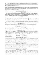
Finally, consider a scheduling objective oriented not to the delays experienced
by customers but rather to the number of jobs waiting in the system at any time. Let
N(t) represent the number of jobs in process (not yet completed) at time t. If we

N(t )

n
(n-1)
(n-2)

2
1

Exhibit 1.4

t


8

K.R. Baker

were to draw a graph of the function N(t), it would resemble the stair-step form of
Exhibit 1.4.
Now suppose that the jobs are sequenced in numerical order (1, 2, …, n) as in
Exhibit 1.4. The function N(t) is level at a height of n for a time interval equal to
the processing time of the first job, or t1. Then the function drops to (n – 1) and
remains level there for a time interval of t2. Then the function drops to (n – 2) and
continues in this fashion, until it eventually drops to zero at time Σ tk. In fact, any
sequence leads to a graph that starts out level at a height of n and eventually drops
to zero at time Σ tk. However, a desirable sequence would be one that tends to keep
N(t) relatively low. To create a specific objective for this goal, we form the time
average of the function N(t), which we can think of as the average inventory. That
is, we weight each value of N(t) by the time this value persists, the values of N(t)
being n, (n – 1), (n – 2), …, 2, 1. In this fashion, we form a weighted sum composed
of the following pairwise products:
n × [length of time N(t) = n]
(n–1) × [length of time N(t) = (n–1]
(n–2) × [length of time N(t) = (n–2)]
...
2 × [length of time N(t) = 2]
1 × [length of time N(t)=1].
The first of these products is the area of the vertical strip in Exhibit 1.4 corresponding to the length of time that there are n jobs in the system. The next product

is the area corresponding to the length of time that there are (n – 1) jobs in the system, and so on. When we sum all the pairwise products (i.e., the areas of the vertical
strips), we obtain the area under the graph of the N(t) function. Then we divide this
sum-of-products by the total time required by the schedule, or Σti, in order to produce the average inventory.
It is not difficult to show that the area under the graph, and therefore the average inventory, is minimized by SPT. Perhaps the quickest way to see this result is
to use the API illustrated in Exhibit 1-3. Suppose that the completion of the “earlier jobs” in the exhibit leaves J jobs in inventory. In schedule S, that leaves J jobs
during the processing of job j and (J – 1) jobs during the processing of job k. In
schedule S’, these numbers are reversed. Now let A represent the contribution of
the earlier and later jobs to the area under the graph. (This contribution is unaffected by the interchange of jobs j and k.) Then we can write:
Area(S) = A + Jtj + (J–1)tk, and


1 Sequencing: The Shortest Processing Time Rule

9

Area(S') = A + Jtk + (J–1)tj .
The difference between the two objectives becomes:
D =Area(S) – Area(S’) = tj–tk.
The area is smaller whenever ∆ > 0, so there will be an improvement whenever
tk < tj. It follows that the minimum possible area (corresponding to the minimum
possible average inventory) is achieved by the SPT sequence.
This derivation shows that shortest-first sequencing minimizes average inventory
as well as average completion time under some very specialized conditions. For example,
the job processing times were assumed to be known with certainty, and all jobs were
available simultaneously. However, the intimate relationship between average inventory
and average completion time holds under many other circumstances. See the coverage
of Little’s Law in Chap. 5 for a broader picture of this relationship.
The dual benefits of SPT sequencing are fortuitous if we think in terms of the
criteria that often guide managers of manufacturing or service systems as they
strive to satisfy a given set of customer orders. One type of concern is the response

time that customers experience. Customers would like delays in satisfying their
orders to be short. As we have seen, if we quantify this concern with the average
completion time objective, an optimal sequencing strategy is shortest-first. Another
type of concern is the pile of unfinished orders in inventory, which managers would
like to keep small. If we quantify this concern with the average inventory objective,
then shortest-first remains an optimal strategy. In the context of our simple sequencing problem, at least, the delay criterion and the inventory criterion may sound quite
different, but they are actually different sides of the same coin: both are optimized
by SPT sequencing. Thus, whether a manager focuses on customer delays or on
unfinished work in progress, or tries to focus on both at once, shortest-first sequencing
is a good idea.

A Generalization of SPT
The shortest-first insights listed in the previous section are useful principles for
making decisions about simple sequencing problems. In practice, there is sometimes a complicating factor: long jobs may often be important ones. Strict priority
in favor of the shortest job would often conflict with importance. How do we reconcile this conflict? In other words, how do we harness the virtues of shortest-first
sequencing while acknowledging that jobs reflect different levels of importance?
To answer this question, we’ll have to go back to our basic problem statement
and enrich it appropriately. To incorporate notions of importance, each job must
have an importance weighting as well as a processing time. Thus, let’s take wi to be
a positive number representing the relative importance (or weight) of the ith job.
(We can think of the values of wi as lying on a scale between zero and one, but the


10

K.R. Baker

scale usually doesn’t matter.) Now the statement of our sequencing problem contains n jobs, each with a given processing time and weight.
Next, we need to specify an objective that is consistent with the use of weights.
An obvious candidate is the weighted sum of completion times. In symbols, the

weighted sum is w1C1 + w2C2 + … + wnCn. This means that, as a result of sequencing choices, each job i experiences a completion time equal to Ci, and we form the
objective by multiplying each completion time by its corresponding weight. Our
objective is to minimize the sum of these values. Shorthand for the weighted sum
of completion times is ΣwC.
To develop a sequencing rule suitable for the weighted objective, we can again investigate adjacent pairwise interchanges. As in Exhibit 1.3, we consider a pair of adjacent
jobs, j and k, somewhere in sequence S, and we swap those two jobs to form the
sequence S'. This time, we let C denote the contributions of the other jobs (excluding j
and k) to the objective, a contribution that is unaffected by the swap, and as before, we
let B denote the time required to complete all the jobs preceding j and k. Then
∑wC(S)=C+wjCj(S)+wkCk(S)=C+wj(B+tj)+wk(B+tj+tk), and
∑wC(S′)=C+wjCj(S′)+wkCk(S′)=C+wj(B+tk+tj)+wk(B+tk).
Then the difference between the two objectives becomes:
D = ∑Ci(S)–∑Ci(S′) = wktj–wjtk.
Since ∆ > 0 if the swap improves the objective, it follows that there will be an
improvement if wjtk < wktj. We can also write this condition as tk/wk < tj/wj. In other
words, the swap improves the objective if it places first the job with the smaller
ratio of processing time to weight. In other words, we can weight each job’s
processing time by dividing it by the job’s weight, then we can sequence the jobs
according to the shortest weighted processing time (SWPT).
Property 1-2. When the objective is the sum of weighted completion times, the
minimum value is achieved by sequencing the jobs in the order of Shortest Weighted
Processing Time.
Property 1-2 reveals that to reconcile the conflict between processing time and
importance weight, we should use the ratio of time to weight. Viewed another way,
the implication is that we should first scale the processing times (divide each one by
its corresponding weight) and then apply the shortest-first principle to the scaled
processing times.
Property 1-2 also applies to situations where the concern is focused on inventory,
but where jobs represent different costs. A common criterion in practice is the minimization of average inventory cost rather than average number of inventory items.
Suppose that each job i has an associated cost, wi. Then a suitable objective could be the

average inventory value, where items are valued at cost. A variation on this objective


1 Sequencing: The Shortest Processing Time Rule

11

V(t)
C1

w1

C2

w2
w3

C3

wn-1

Cn-1
wn

Cn
t

Exhibit 1.5
is to value items at some percentage of cost that reflects the opportunity cost of carrying stock. At the outset, all jobs are in inventory, so the inventory value is Σwi. As jobs
in the sequence are finished, the value of inventory drops, eventually falling to zero.

A graphical representation is shown in Exhibit 1.5, where the graph tracks
the value of inventory V(t) over time. For the purpose of illustration, suppose
the jobs are sequenced in numerical order. Then the inventory value is Σwi for
a time interval equal to the processing time of the first job. At that point, the
inventory value drops by w1 and remains at that level until the second job completes.
The graph follows a stair-step pattern, but in contrast to Exhibit 1.4, the step
sizes are not all the same. Each step down corresponds to a reduction in inventory value by one of the wi values. Again, the objective is the minimize the area
under the graph of V(t), and again, we can show that this objective is achieved
by the SWPT sequence.

Shortest-First and Group Technology
An important principle in organizing systems with many elements is to group like
elements together. Elaborating on this idea, the group technology principle has
been applied effectively in discrete-parts manufacturing. For example, parts can be
grouped in to similar families according shapes, sizes, materials, etc. In many manufacturing applications, a machine switches from making products of one family to
making products of another family by means of an expensive setup. To avoid excessive setup time, and to simplify scheduling, many production schedules allow just
one setup for all the parts in each product family. The jobs in the family are then


12

K.R. Baker

grouped together so that they can all be done after the same setup. How does the
shortest-first principle apply to a sequence of groups?
In the so-called group technology problem, the given information consists of a
set of jobs, the family each belongs to, their processing times, and their weights.
For family f, let Tf represent the sum of the processing times of all the jobs in the
family, let Wf represent the sum of the weights, and let sf represent the length of the
setup time required to begin production of the family. Then, to solve the problem

of minimizing ΣwC, the first step is to sequence the jobs by SWPT within families.
Then, to order the families, choose according to the smallest ratio (sf + Tf)/Wf. In
effect, this prescription implements SWPT twice. At the level of jobs, the sequencing rule holds, in its usual form. At the level of families, the sequencing rule applies
to family processing time (including setup), as scaled by total family weight.

Limitations of APIs
We have seen that the shortest-first rule yields an optimal sequence when we are interested
in simple measures of delay. That is, if the objective is the sum of completion times or the
sum of wait times, we know that shortest-first priority is optimal. We also know that this
principle generalizes to importance weights if we scale the processing times. Furthermore,
an adaptation of the shortest-first rule applies to jobs when they are grouped in families.
We might wonder when the shortest-first rule would fail.
As an illustration of the limits of SPT sequencing, consider a situation in which
jobs have due dates but no weights. In other words, the given information consists
of n, the number of jobs, and, for each job, a processing time ti and a due date di.
The presence of due dates gives rise to a scheduling goal that is different from minimizing delay times or inventory costs. When due dates exist, a reasonable goal is
completing jobs by their due dates. One way to quantify this goal is to calculate a
tardiness value for each job in the schedule. Tardiness is defined as Ti = max{0, Ci – di}.
In other words, tardiness is zero as long as job i completes by its due date; otherwise,
tardiness is equal to the amount of time that the job is late. A reasonable objective
is to minimize the sum of tardiness values in a sequence, for which the usual shorthand is ΣT. If we can work to this objective, then whenever there is a sequence that
completes all jobs on time, we could produce it by using ΣT as an objective and
finding its minimum value.
However, finding the minimum value of ΣT is not a straightforward problem. To
suggest why this is so, let us return to the method of adjacent pairwise interchanges.
Specifically, we consider swapping jobs j and k as in Exhibit 1.3, but now with the
ΣT objective in mind. In addition, take job k to be shorter than job j, so that tk < tj.
Consider the situation depicted in Exhibit 1.6, where job j is originally on time and
k is late in schedule S. After the swap, job k is on time and j is late. However, the
increase in the tardiness of job j (rightward arrow) is greater than the decrease in

the tardiness of job k (leftward arrow), as the example is constructed, so that the
swap actually makes the total tardiness worse.