Thermal analysis fundamentals and applications to polymer science hatakeyama, t quinn, f x

Document

Page iii

Thermal Analysis
Fundamentals and Applications to Polymer Science
Second Edition
T. Hatakeyama
Otsuma Women's University, Faculty of Home Economics, Tokyo, Japan
F.X. Quinn
L'Oréal Recherche Avancée, Aulnay-sous-Bois, France

file:///Q|/t_/t_iii.htm2/10/2006 11:33:34 AM


Document

Page iv

Copyright © 1999 by John Wiley & Sons Ltd.
Baffins Lane, Chichester,
West Sussex PO19 IUD, England
National 01243 779777
International (+44) 1243 779777
e-mail (for orders and customer service enquiries): cs-books @ wiley.co.uk
Visit our Home Page on or
All Rights Reserved. No part of this publication may be reproduced, stored in a retrieval system, or
transmitted, in any form or by any means, electronic, mechanical, photocopying, recording, scanning or
otherwise, except under the terms of the Copyright, Designs and Patents Act 1988 or under the terms of
a licence issued by the Copyright Licensing Agency, 90 Tottenham Court Road, London, W1P 9HE,

UK, without the prior permission in writing of the publisher.
Other Wiley Editorial Offices
John Wiley & Sons, Inc. , 605 Third Avenue,
New York, NY 10158-0012, USA
WILEY-VCH Verlag GmbH, Pappelallee 3,
D-69469 Weinheim, Germany
Jacaranda Wiley Ltd. 33 Park Road, Milton,
Queensland 4064, Australia
John Wiley & Sons (Asia) Pte Ltd, 2 Clementi Loop #02 01,
Jin Xing Distripark, Singapore 129809
John Wiley & Sons (Canada) Ltd, 22 Worcester Road,
Rexdale, Ontario M9W ILI, Canada
Library of Congress Cataloging-in-Publication Data
Hatakeyama, T.
Thermal analysis: fundamentals and applications to polymer
science/ T. Hatakeyama, F.X. Quinn. —2nd ed.
p. cm.
Includes bibliographical references and indexes.
ISBN 0-471-98362-4 (hb)
1. Thermal analysis. 2. Polymers—Analysis. I. Quinn, F.X.
II. Title.
QD79.T38H38
1999
543'.086—dc21
98-49129
CIP
British Library Cataloguing in Publication Data
A catalogue record for this book is available from the British Library
ISBN 0 471 98362 4
Typeset in 10/12pt Times New Roman by Pure Tech India Ltd, Pondicherry

Printed and bound in Great Britain by Biddles Limited, Guildford, Surrey
This book is printed on acid-free paper responsibly manufactured from sustainable forestry, in which at
least two trees are planted for each one used for paper production.

file:///Q|/t_/t_iv.htm2/10/2006 11:33:46 AM


Document

Page v

Contents
Preface

ix

Preface to the Second Edition

x

1
Thermal Analysis

1

1.1 Definition

1

1.2 Characteristics of Thermal Analysis

2

1.3 Conformation of Thermal Analysis Instruments

3

1.4 Book Outline

4

2
Differential Thermal Analysis and Differential Scanning Calorimetry
2.1 Differential Thermal Analysis (DTA)
2.1.1 Custom DTA
2.2 Quantitative DTA (Heat-Flux DSC)

5

5
7
8

2.3 Triple-Cell Quantitative DTA

10

2.4 Power Compensation Differential Scanning Calorimetry (DSC)

11

2.5 Temperature Modulated DSC (TMDSC)

12

2.5.1 General Principles of Temperature Modulated DSC

13

2.5.2 TMDSC Calibration

18

2.5.3 TMDSC Experimental Conditions

18

2.6 High-Sensitivity DSC (HS-DSC)

20

2.7 Data Analysis and Computer Software

21

2.8 Automated TA Systems

22

2.9 Simultaneous TA

22

2.10 Installation and Maintenance

22

2.11 References

24

3
Calibration and Sample Preparation
3.1 Baseline

25

25

3.1.1 Baseline Curvature and Noise

25

3.1.2 Baseline Subtraction

27

3.1.3 Baseline Correction

28

3.2 Temperature and Enthalpy Calibration

28

3.3 Sample Vessel

29

3.4 Sample Preparation

32

file:///Q|/t_/t_v.htm2/10/2006 11:33:48 AM


Document

Page vi

3.4.1 Films, Sheets and Membranes

33

3.4.2 Granules and Blocks

34

3.4.3 Powders

34

3.4.4 Fibres and Fabrics

34

3.4.5 Biomaterials and Gels

35

3.4.6 Storing Samples

35

3.5 Temperature Gradient in Sample

36

3.5.1 Mass of Sample

37

3.5.2 Solutions

39

3.6 Sample Packing

39

3.6.1 Hydrophilic Sample

40

3.6.2 Liquid Sample

40

3.7 Purge Gas

41

3.8 Scanning Rate

41

3.9 Sub-ambient Operation

43

4
Thermogravimetry

45

4.1 Introduction

45

4.2 Thermobalance

46

4.2.1 Installation and Maintenance

46

4.2.2 Microbalance and Crucible

47

4.2.3 Furnace and Temperature Programmer

50

4.2.4 Data Recording Unit

54

4.3 Temperature Calibration

55

4.4 Sample

58

4.5 Atmosphere

61

4.6 Heating Rate

63

4.7 Classification of TG Curves

65

4.8 Calculation of Mass Change Rates

66

4.9 Derivative Thermogravimetry (DTG)

68

4.10 Intercomparison of TG and DTA

68

4.11 TG Reports

70

4.12 References

71

5

Applications of Thermal Analysis

72

5.1 Temperature Measurement

72

5.2 Enthalpy Measurement

74

5.2.1 Polymer Melting (Initial Crystallinity)
5.3 Reaction Rate Kinetics

75
77

5.3.1 Differential Methods

80

5.3.2 Integral Methods

82

5.3.3 Jump Method

84

5.3.4 Isothermal Crystallization of Polymers

85

5.3.5 General Comment on Reaction Rate Kinetics

88

file:///Q|/t_/t_vi.htm (1 of 2)2/10/2006 11:34:00 AM


Document

Page vii

5.4 Glass Transition of Polymers

90

5.4.1 Enthalpy Relaxation of Glassy Polymers

91

5.4.2 Enthalpy Relaxation Measurement by TMDSC

95

5.4.3 Glass Transition Measurement by TMDSC

95

5.4.4 Glass Transition in the Presence of Water

96

5.5 Heat Capacity Measurement by DSC

97

5.6 Heat Capacity Measurement by TMDSC

100

5.7 Purity Determination by DSC

102

5.7.1 Thermal Lag

103

5.7.2 Undetected Premelting

103

5.7.3 General Comment on Purity Determination by DSC

104

5.8 Crystallinity Determination by DSC

105

5.9 Molecular Rearrangement during Scanning

106

5.10 Polymorphism

107

5.11 Annealing

109

5.12 Bound Water Content

109

5.12.1 Experimental Procedure

112

5.13 Phase Diagram

113

5.14 Gel-Sol Transition

115

5.14.1 Other Applications of HS-DSC
5.15 References

117
118

6
Other Thermal Analysis Methods

119

6.1 Evolved Gas Analysis

119

6.1.1 Mass Spectrometry (MS)

119

6.1.2 Fourier Transform Infrared (FTIR) Spectroscopy

120

6.1.3 Gas Chromatography (GC)

121

6.1.4 TG-EGA Report

123

6.2 Mechanical Analysis

125

6.2.1 Thermomechanical Analysis (TMA)

126

6.2.2 Dynamic Mechanical Analysis (DMA)

130

6.2.3 TMA and DMA Reports

133

6.3 Dilatometry

133

6.3.1 Dilatometer Assembly

133

6.3.2 Definition of Expansion Coefficients

135

6.4 Thermomicroscopy

136

6.4.1 Observation by Reflected Light

137

6.4.2 Observation by Transmitted Light

137

6.5 Simultaneous DSC-X-Ray Analysis

139

6.6 Thermoluminescence (TL)

139

6.7 Alternating Current Calorimetry (ACC)

142

6.8 Thermal Diffusivity (TD) Measurement by Temperature Wave Method

145

6.9 Thermally Stimulated Current (TSC)

148

file:///Q|/t_/t_vii.htm (1 of 2)2/10/2006 11:34:03 AM


Document

Page viii

6.10 Thermal Conductivity

152

6.11 Micro-thermal Analysis (µTA)

153

6.12 Optothermal Transient Emission Radiometry (OTTER)

154

6.13 Specific Heat Spectroscopy

155

6.14 References

156

Appendix 1

Glossary of TA Terms

158

Appendix 2
Standard Reference Materials

164

Appendix 3
Physical Constants and Conversion Tables

167

Chemical Formula Index

172

Subject Index

175

file:///Q|/t_/t_viii.htm2/10/2006 11:34:11 AM


Document

Page ix

Preface

We are grateful to those many friends, M. Maezono, Z. Liu, K. Nakamura, T. Hashimoto, S. Hirose, H.
Yoshida and C. Langham, whose considerable input helped us to write this book.
We would like to extend special thanks to Hyoe Hatakeyama, who made many valuable suggestions
when authors from different backgrounds encountered various problems. Without his encouragement
this book could not have been written.
The book is the result of the merging of ideas from both East and West. We hope that readers will find
it useful in their work. As Confucius said, it is enjoyable when friends come from far places and work
together for the same purpose.
TSUKUBA
JUNE, 1994

file:///Q|/t_/t_ix.htm2/10/2006 11:34:13 AM

T.H.
F.X.Q.


Document

Page x

Preface to the Second Edition
The principle motivation behind the revision of this book resides in the burgeoning interest in
temperature modulated thermal analysis methods. In this revised edition the sections on temperature
modulated thermal analysis have been updated and considerably increased in size. We greatefully
acknowledge stimulating discussions on TMDSC with Leonard C. Thomas and Marine Peron.
In response to criticism from members of the electronics industry that thermal analysis methods are
often incompatible with the rapid pace of corporate research & development, new sections have been
introduced on thermally stimulated current spectroscopy, thermal conductivity, optothermal transient
emission radiometry and micro-thermal analysis (µTA).

It is our belief that thermal analysis can be of great value in industrial applications, but in keeping with
the spirit of this text the limitations as well as the advantages of thermal analysis are presented and
discussed.
TH (TOKYO)
FXQ (PARIS)
JANUARY 1999

file:///Q|/t_/t_x.htm2/10/2006 11:34:14 AM


Document

Page 1

1—
Thermal Analysis
1.1 Definition
The term thermal analysis (TA) is frequently used to describe analytical experimental techniques which
investigate the behaviour of a sample as a function of temperature. This definition is too broad to be of
practical use. In this book, TA refers to conventional TA techniques such as differential scanning
calorimetry (DSC), differential thermal analysis (DTA), thermogravimetry (TG), thermomechanical
analysis (TMA) and dynamic mechanical analysis (DMA). A selection of representative TA curves is
presented in Figure 1.1.
TA, in its various guises, is widely employed in both scientific and industrial domains. The ability of
these techniques to characterize, quantitatively and

Figure 1.1.
Representative TA curves

file:///Q|/t_/t_1.htm2/10/2006 11:08:48 AM

Document

Page 2

qualitatively, a huge variety of materials over a considerable temperature range has been pivotal in their
acceptance as analytical techniques. Under normal conditions only limited training of personnel is
required to operate a TA instrument. This, coupled with the fact that results can be obtained relatively
quickly, means that TA is employed in an ever increasing range of applications. However, the
operational simplicity of TA instruments belies the subtlety of techniques which, if improperly
practised, can give rise to misleading or erroneous results. The abundance of results of dubious integrity
in both the academic literature and industrial performance reports underlines the extent and seriousness
of this problem.
1.2 Characteristics of Thermal Analysis
The advantages of TA over other analytical methods can be summarized as follows: (i) the sample can
be studied over a wide temperature range using various temperature programmes; (ii) almost any
physical form of sample (solid, liquid or gel) can be accommodated using a variety of sample vessels or
attachments; (iii) a small amount of sample (0.1 µg-10 mg) is required; (iv) the atmosphere in the
vicinity of the sample can be standardized; (v) the time required to complete an experiment ranges from
several minutes to several hours; and (vi) TA instruments are reasonably priced. In polymer science,
preliminary investigation of the sample transition temperatures and decomposition characteristics is
routinely performed using TA before spectroscopic analysis is begun.
TA data are indirect and must be collated with results from spectroscopic measurements [for example
NMR, Fourier transform infrared (FTIR) spectroscopy, X-ray diffractometry] before the molecular
processes responsible for the observed behaviour can be elucidated. Irrespective of the rate of
temperature change, a sample studied using a TA instrument is measured under nonequilibrium
conditions, and the observed transition temperature is not the equilibrium transition temperature. The
recorded data are influenced by experimental parameters, such as the sample dimensions and mass, the
heating/cooling rate, the nature and composition of the atmosphere in the region of the sample and the

thermal and mechanical history of the sample. The precise sample temperature is unknown during a TA
experiment because the thermocouple which measures the sample temperature is rarely in direct contact
with the sample. Even when in direct contact with the sample, the thermocouple cannot measure the
magnitude of the thermal gradients in the sample, which are determined by the experimental conditions
and the instrument design. The sensitivity and precision of TA instruments to the physicochemical
changes occurring in the sample are relatively low compared with spectroscopic techniques. TA is not a
passive experimental method as the high-order structure of a sample (for example crystallinity, network
formation, morphology) may change during the measurement. On the other hand, samples can be

file:///Q|/t_/t_2.htm2/10/2006 11:09:08 AM


Document

Page 3

annealed, aged, cured or have their previous thermal history erased using these instruments.
1.3 Conformation of Thermal Analysis Instruments
The general conformation of TA apparatus, consisting of a physical property sensor, a controlled-atmosphere
furnace, a temperature programmer and a recording device, is illustrated in Figure 1.2. Table 1.1 lists the most
common forms of TA. Modern TA apparatus is generally interfaced to a computer (work station) which
oversees operation of the instrument controlling the temperature range, heating and cooling rate, flow of purge
gas and data accumulation and storage. Various types of data analysis can be performed by the computer. A
trend in modern TA is to use a single work station to operate several instruments simultaneously (Figure 1.3).
TA apparatus without computers is also used where the analogue output signal is plotted using a chart recorder.
Data are accumulated on chart paper and calculations performed manually. The quality of the data obtained is
not diminished in any way. The accuracy of the results is the same provided that the apparatus is used properly
and the data are analysed correctly. Some in

Figure 1.2.

Block diagram of TA instrument
Table 1.1. Conventional forms of TA
Property

TA method

Abbreviation

Mass

Thermogravimetry

Difference temperature

Differential thermal analysis

DTA

Alternating temperature

Alternating current calorimetry

ACC

Enthalpy

Differential scanning calorimetry

DSC

Length, volume

Dilatometry

Deformation

Thermomechanical analysis

TMA

Dynamic mechanical analysis

DMA

Electric current

Thermostimulated current

TSC

Luminescence

Thermoluminescence

file:///Q|/t_/t_3.htm2/10/2006 11:09:18 AM

TG

TL

Document

Page 4

Figure 1.3.
Simultaneous operation of several TA
instruments using a central work station

struments are equipped with both a computer and a chart recorder in order, for example, to evaluate
ambiguous shifts in the sample baseline.
1.4 Book Outline
This text is designed to acquaint and orientate newcomers with TA by providing a concise introduction
to the basic principles of instrument operation, advice on sample preparation and optimization of
operating conditions and a guide to interpreting results. The text deals with DSC and DTA in Chapters
2 and 3. TG is described in Chapter 4. In Chapter 5 the application of these TA techniques to polymer
science is presented. Other TA techniques are briefly described for completeness in Chapter 6. The
Appendices include a glossary of TA terms, a survey of standard reference materials and TA conversion
tables.
Although primarily pitched at newcomers, this book is also intended as a convenient reference guide for
more experienced users and to provide a source of useful TA information for professional thermal
analysts.

file:///Q|/t_/t_4.htm2/10/2006 11:09:26 AM


Document

Page 5

2—
Differential Thermal Analysis and Differential Scanning Calorimetry
2.1 Differential Thermal Analysis (DTA)
The structure of a classical differential thermal analyser is illustrated in Figure 2.1. The sample holder
assembly is placed in the centre of the furnace. One holder is filled with the sample and the other with
an inert reference material, such as α-alumina. The term 'reference material' used in TA is frequently
confused with the term 'standard reference material' used for calibration, since in many other analytical
techniques the same material is used for both purposes. However, a reference material in TA is a
thermally inert substance which exhibits no phase change over the temperature range of the experiment.
Thermocouples inserted in each holder measure the temperature difference between the sample and the
reference as the temperature of the furnace is controlled by a temperature programmer. The temperature
ranges and

Figure 2.1.
Schematic diagram of
classical DTA apparatus

file:///Q|/t_/t_5.htm2/10/2006 11:09:30 AM


Document

Page 6
Table 2.1. Thermocouples commonly used in DTA
Thermocouple

Electric terminal

Recommended
operating range/K

+

-

Cu-Constantana

Cu

Constantan

90-600

Chromelb-Constantan

Chromel

Constantan

90-1000

Chromel-Alumelc

Chromel

Alumel

270-1300

Pt-Pt/Rhd

Pt/Rh

Pt

500-1700

a Constantan:
b Chromel:
c Alumel:
d

Cu 60-45%, Ni 40-55%.

Ni 89%, Cr 9.8%, trace amounts of Mn and Si2 O3 .

Ni 94%, Mn 3%, Al 2%, Si2 O3 1%.

Pt/Rh: Pt 90%, Rh 10%.

compositions of commonly used thermocouples are listed in Table 2.1. The thermocouple signal is of the order of
millivolts.
When the sample holder assembly is heated at a programmed rate, the temperatures of both the sample and the
reference material increase uniformly. The furnace temperature is recorded as a function of time. If the sample
undergoes a phase change, energy is absorbed or emitted, and a temperature difference between the sample and the
reference (∆T) is detected. The minimum temperature difference which can be measured by DTA is 0.01 K.
A DTA curve plots the temperature difference as a function of temperature (scanning mode) or time (isothermal
mode). During a phase transition the programmed temperature ramp cannot be maintained owing to heat absorption
or emission by the sample. This situation is illustrated in Figure 2.2, where the temperature of the sample holder
increases above the programmed value during crystallization owing to the exothermic heat of crystallization. In

Figure 2.2.
Schematic illustration of the
measured sample temperature as
a function of time for a polymer
subjected to a linear heating ramp,
and the corresponding DTA curve. In
the region of the phase transitions the
programmed and measured sample
temperatures deviate significantly

file:///Q|/t_/t_6.htm2/10/2006 11:09:31 AM


Document

Page 7

contrast, during melting the temperature of the sample holder does not increase in response to the
temperature programmer because heat flows from the sample holder to the sample. Therefore, the true
temperature scanning rate of the sample is not constant over the entire temperature range of the
experiment.
Temperature calibration is achieved using standard reference materials whose transition temperatures
are well characterized (Appendices 2.1 and 2.2) and in the same temperature range as the transition in
the sample. The transition temperature can be determined by DTA, but the enthalpy of transition is
difficult to measure because of non-uniform temperature gradients in the sample due to the structure of
the sample holder, which are difficult to quantify. This type of DTA instrument is rarely used as an
independent apparatus and is generally coupled to another analytical instrument for simultaneous
measurement of the phase transitions of metals and inorganic substances at temperatures greater than
1300 K.

2.1.1 Custom DTA
Many DTA instruments are constructed by individual researchers to carry out experiments under
specialized conditions, such as high pressure and/or high temperature. Figure 2.3 shows an example of a
high-pressure custom DTA instrument. The pressure medium used is dimethylsilicone (up to 600 MPa)
or kerosene (up to 1000 MPa) and the pressure is increased using a mechanical or

Figure 2.3.
Schematic diagram of a high-pressure
custom DTA apparatus (courtesy of Y. Maeda)

file:///Q|/t_/t_7.htm2/10/2006 11:09:34 AM


Document

Page 8

Figure 2.4.
DTA heating curves of
polyethylene recorded at various
pressures. (I) 0.1, (II) 200,
(III) 250 and (IV) 350 MPa
(courtesy of Y. Maeda)

an electrical pump. The temperature range is 230-670 K at a heating rate of 1-5 K/min. The pressure
range of commercially available high-pressure DTA systems is 1-10 MPa to guarantee the stability and
safety of the apparatus. In this case, the excess pressure is generated using a purge gas (CO2 , N2 , O2 ).
The DTA heating curves of polyethylene measured over a range of pressures are presented in Figure 2.4.
DTA systems capable of measuring large amounts of sample (> l00g) have been constructed to analyse
inhomogeneous samples such as refuse, agricultural products, biowaste and composites.

2.2 Quantitative DTA (Heat-Flux DSC)
The term heat-flux differential scanning calorimeter is widely used by manufacturers to describe
commercial quantitative DTA instruments. In quantitative DTA, the temperature difference between the
sample and reference is measured as a function of temperature or time, under controlled temperature
conditions. The temperature difference is proportional to the change in the heat flux (energy input per
unit time). The structure of a quantitative DTA system is shown in Figure 2.5. The conformation of the
sample holder assembly is different from that in a classical DTA set-up. The thermocouples are
attached to the base of the sample and reference holders. A second series of thermocouples measures
the temperature of the furnace and of the heat-sensitive plate. During a phase change heat is absorbed or
emitted by the sample, altering the heat flux through the heat-sensitive plate. The variation in heat flux
causes an incremental temperature difference to be measured between the heat-sensitive plate and the
furnace. The heat capacity of the heat-sensitive plate as a function

file:///Q|/t_/t_8.htm2/10/2006 11:09:40 AM


Document

Page 9

Figure 2.5.
(A) Schematic diagram of quantitative DTA apparatus;
(B) TA Instruments design (by permission of TA Instruments);
(C) Seiko Instruments design (by permission of Seiko Instruments)

file:///Q|/t_/t_9.htm2/10/2006 11:09:43 AM


Document

Page 10

of temperature is measured by adiabatic calorimetry during the manufacturing process, allowing an
estimate of the enthalpy of transition to be made from the incremental temperature fluctuation. The
sample and reference material are placed in sample vessels and inserted into the sample and reference
holders. For optimum performance of a quantitive DTA system the sample should weigh < 10 mg, be as
flat and thin as possible and be evenly placed on the base of the sample vessel. The maximum
sensitivity of a quantitative DTA instrument is typically 35 µ W.
The furnace of a quantitative DTA system is large and some designs can be operated at temperatures
greater than 1000 K. When the sample holder is constructed from platinum or alumina the maximum
operating temperature is approximately 1500 K. A linear instrument baseline can be easily obtained
because the large furnace heats the atmosphere surrounding the sample holder. The outside of the
sample holder assembly casing can become very hot during operation and should be handled with care,
even after the instrument has finished a scan. Moisture does not condense on the sample holder in
subambient mode because of the large heater, making adjustment of the instrument baseline at low
temperatures relatively easy.
The time needed to stabilize a quantitive DTA instrument at an isothermal temperature is long for both
heating and cooling. For example, when cooling at the maximum programmed rate from 770 to 300 K
approximately 30-100s are required before the temperature equilibrates. To avoid overshooting the
temperature on heating the constants of the PID (proportional integral differential) temperature control
programme must be adjusted, especially for isothermal experiments where the scanning rate to the
isothermal temperature is high. Overshooting also makes heat capacity measurements difficult. The
temperature difference between the furnace and the sample can be very large on heating and cooling,
particularly if a high scanning rate is used. Instruments are generally constructed so that when the
furnace temperature is equal to the selected final temperature the scan is terminated. The sample
temperature may be well below this value, and from the point of view of the user the experiment is
prematurely terminated. It is recommended to verify the difference between the furnace and sample
temperature under the proposed experimental conditions before beginning analysis.
2.3 Triple-Cell Quantitative DTA
At high temperatures the effect of radiative energy from the furnace can no longer be neglected as this

contribution increases as T4. Triple-cell DTA systems have been constructed, using the same principle
as quantitative DTA, to measure accurately the enthalpy of transition at temperatures greater than 1000
K (Figure 2.6) [1]. A vacant sample vessel, the sample and a reference material are measured
simultaneously. The repeatability of the DTA curve with this instrument is ±3% up to 1500 K. The
radiative effect is alleviated by

file:///Q|/t_/t_10.htm2/10/2006 11:10:05 AM


Document

Page 11

Figure 2.6.
Schematic diagram of triple-cell DTA system. Hightemperature enthalpy measurements are more precise with this
instrument as compared with standard quantitative DTA systems.
(Reprinted from Y. Takahachi and M. Asou, Thermochimica Acta.
223, 7, 1993, with permission from Elsevier Science)

placing three high thermal conductivity adiabatic walls between the furnace and the sample holder
assembly.
2.4 Power Compensation Differential Scanning Calorimetry (DSC)
A power compensation-type differential scanning calorimeter employs a different operating principle
from the DTA systems presented earlier. The structure of a power compensation-type DSC instrument
is shown in Figure 2.7. The base of the sample holder assembly is placed in a reservoir of coolant. The
sample and reference holders are individually equipped with a resistance sensor, which measures the
temperature of the base of the holder, and a resistance heater. If a temperature difference is detected
between the sample and reference, due to a phase change in the sample, energy is supplied until the
temperature difference is less than a threshold value, typically < 0.01 K. The energy input per unit time
is recorded as a function of temperature or time. A simplified consideration of the thermal properties of

this configuration shows that the energy input is proportional to the heat capacity of the sample. The
maximum sensitivity of this instrument is 35 µ W.
The temperature range of a power compensation DSC system is between 1 10 and 1000 K depending on
the model of sample holder assembly chosen. Some units are only designed to operate above 290 K,
whereas others can be used over the entire temperature range. Temperature and energy calibration are
achieved using the standard reference materials in Appendix 2.1. The heater of a power compensationtype DSC instrument is smaller than that of a quantitative DTA apparatus, so that the temperature
response is quicker and higher scanning rates can be used. Instruments display scanning rates from 0.3
to 320 K/min on heating and cooling. The maximum reliable scanning rate is 60 K/min. Isothermal
experiments, annealing (single- and multi-step) and heat

file:///Q|/t_/t_11.htm2/10/2006 11:10:06 AM


Document

Page 12

Figure 2.7.
(A) Block diagram and (B) schematic diagram of power
compensation DSC system (by permission of Perkin-Elmer Corp.)

capacity measurements can be performed more readily using the power compensation-type instrument.
Maintaining the instrument baseline linearity is a problem at high temperatures or in the sub-ambient
mode. Moisture condensation on the sample holder must be avoided during sub-ambient operation.
2.5 Temperature Modulated DSC (TMDSC)
A variation on the standard temperature programmes used in TA has recently been introduced [2-6].
This technique can in principle be applied to quantitative

file:///Q|/t_/t_12.htm2/10/2006 11:10:06 AM

Document

Page 13

DTA as well as power compensation DSC instruments, and is called temperature modulated DSC, or
TMDSC. The following trade marks are used by different TA instrument manufacturers for their
temperature modulated differential scanning calorimeters: Modulated DSCTM (MDSCTM) of TA
Instruments Inc. , Oscillating DSCTM (ODSCTM) of Seiko Instruments Inc. , Alternating DSCTM
(ADSCTM) of Mettler-Toledo Inc. and Dynamic DSCTM (DDSCTM) of Perkin-Elmer Corp.
2.5.1 General Principles of Temperature Modulated DSC
Temperature modulated DSC (TMDSC) can most readily be understood by comparing it to
conventional DSC. As described in Section 2.2, in a quantitative DTA (heat-flux DSC) the difference in
heat flow between a sample and an inert reference material is measured as a function of time as both the
sample and reference are subjected to a controlled temperature profile. The temperature profile is
generally linear (heating or cooling), varying in range from 0 K/ min (isothermal) to 60 K/min. Thus the
programmed sample temperature, T(t) is given by

where T0 (K), β (K/min) and t (min) denote the starting temperature, linear constant heating (or cooling)
rate and time, respectively.
Temperature modulated DSC uses the heat-flux DSC instrument design and configuration to measure
the differential heat flow between a sample and an inert reference material as a function of time.
However, in TMDSC a sinusoidal temperature modulation is superposed on the linear (constant)
heating profile to yield a temperature programme in which the average sample temperature varies
continuously in a sinusoidal manner:

where AT (±K) denotes the amplitude of the temperature modulation, ω (s-1) is the modulation
frequency and ω = 2π/p, where p (s) is the modulation period.
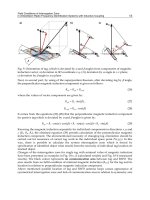
Figure 2.8 illustrates a modulated temperature profile for a TMDSC heating experiment, which is
equivalent by decomposition to applying two profiles simultaneously to the sample: a linear (constant)

heating profile and a sinusoidal heating profile. The temperature profiles of these two simultaneous
experiments are governed by the following experimental parameters:
ã constant heating rate (ò = 0-60 K/min);
• modulation period (p= 10-100 s);
• temperature modulation amplitude (AT = ± 0.01-10 K).
The total heat flow at any point in a DSC or TMDSC experiment is given by

file:///Q|/t_/t_13.htm2/10/2006 11:10:07 AM


Document

Page 14

Figure 2.8.
Typical TMDSC heating profile with the
following experimental parameters: ß = 1 K/min,
p = 30 s and AT = ±1 K. Under these conditions
the instantaneous heating profile varies between 13.5
and -11.5 K/min, and thus cooling occurs during a
portion of the temperature modulation. The
maximum/minimum instantaneous heating rate is
calculated using ßmax/min = (60 x 2π x AT x 1/p) + ß
(courtesy of TA Instruments Inc.)

where Q (J) denotes heat, t (s) time, Cp (J/K) sample heat capacity and ƒ(T,t) the heat flow from kinetic
processes which are absolute temperature and time dependent.
Conventional DSC only measures the total heat flow. TMDSC also measures the total heat flow, but by
effectively applying two simultaneous temperature profiles to the sample can estimate the individual
contributions to equation 2.3. The constant heating profile (dashed line in Figure 2.8) provides total heat

flow information while the sinusoidal heating profile (solid line in Figure 2.8) gives heat capacity
information corresponding to the rate of temperature change. The heat capacity component of the total
heat flow, Cp ß, is generally referred to as the reversing heat flow and the kinetic component, ƒ(T, t), is
referred to as the non-reversing heat flow.
TMDSC data are calculated from three measured signals: time, modulated heat flow and modulated
heating rate (the derivative of modulated temperature). The raw data are visually complex and require
deconvolution to obtain standard DSC curves. However, raw data are useful for revealing the sample
behaviour during temperature modulation, as well as fine-tuning experimental conditions and detecting
artefacts.
As described in Section 5.5, the sample heat capacity is generally estimated in conventional DSC from
the difference in heat flow between the sample and an empty sample vessel, using sapphire as a
calibrated reference material. Alternatively, Cp can be determined from the difference in heat flow
between two scans on identical samples at two different heating rates.

file:///Q|/t_/t_14.htm2/10/2006 11:10:08 AM


Document

Page 15

In TMDSC the heating rate changes during the modulation cycle, so that dividing the difference in
modulated heat flow by the difference in the modulated heating rate is equivalent to the conventional
DSC two heating rates method. The heat capacity is calculated using a discrete Fourier transformation
and is given qualitatively by

where K denotes the heat capacity calibration constant, Qamp the heat flow amplitude and Tamp the
temperature amplitude. Applying a Fourier transformation implicitly assumes that the superposition
principle is valid in the sample [7]. In the case of TMDSC this is true for baseline and peak area
measurements, and thus TMDSC can be used for measuring Cp .

The total, reversing and non-reversing heat flow curves of a quenched poly(ethylene terephthalate)
(PET) sample are presented in Figure 2.9. The total heat flow is calculated as the average of the
modulated heat flow (Figure 2.9A). The modulated signal is not corrected real-time and transitions in
the modulated signal appear to be shifted to lower temperatures compared to the averaged data. This
apparent shift is due to delays associated with real-time deconvolution and smoothing, and is generally
about 1.5 cycles.
The reversing component of the total heat flow signal is equal to Cp ß. The non-reversing component is
the arithmetic difference between the total heat flow and the reversing component:

The separation of the total heat flow into its reversing and non-reversing components is affected by
experimental conditions, particularly when time-dependent (non-reversing) phenomena occur. Timedependent effects may occur in polymer samples due to their low thermal conductivies or in samples
undergoing fusion[8]. Controlled temperature modulation cannot be maintained throughout melting
because the modulation heating rate increases dramatically as melting reaches a maximum. The effect is
amplified as the sample purity increases, so that the temperature of a pure substance (for example,
indium) cannot be modulated. In the absence of controlled temperature modulation the heat capacity
can no longer be measured, and so neither the reversing nor the non-reversing heat flow can be
determined. Note that the total heat flow signal is quantitatively correct regardless of the modulation
conditions. Guidelines for ensuring and monitoring correct temperature modulation of the sample will
be presented in Section 2.5.3.
By separating the individual heat flow components TMDSC can be used to distinguish overlapping
thermal events with different behaviours. Figure 2.10A shows a DSC curve of the first heat of a PET/
acrylonitrile-butadiene-styrene (ABS) blend. Three transitions associated with the PET phase are
observed:

file:///Q|/t_/t_15.htm2/10/2006 11:10:09 AM


Document

Page 16

Figure 2.9.
(A) Total heat flow signal (raw and averaged data)
for a sample of quenched PET. (B) Total, reversing and nonreversing heat flow averaged signals for a sample of quenched
PET. Experimental parameters: sample mass 5.5 mg,
ß = 2 K/min, p = 100 s and AT = ±l K
(courtesy of TA Instruments Inc.)

glass transition (340 K), cold crystallization (394 K) and fusion (508 K). No apparent ABS transitions
are observed. Following cooling at 10 K/min the blend is reheated and two transitions are observed:
glass transition (379 K) and fusion (511 K).
TMDSC first heating curves for an identical sample of the blend are presented in Figure 2.10B. The
exotherm associated with PET cold crystallization and a small endotherm at 343 K associated with
relaxation phenomena are revealed in the non-reversing signal. Two glass transitions, ascribed to PET
at 340 K and to ABS at 378 K, are found in the reversing signal. In conventional DSC the latter glass
transition is hidden beneath the PET cold crystallization

file:///Q|/t_/t_16.htm2/10/2006 11:10:10 AM