VẬT lý địa CHẤN 04 velocity
Bạn đang xem bản rút gọn của tài liệu. Xem và tải ngay bản đầy đủ của tài liệu tại đây (347.78 KB, 21 trang )
Seismic Velocities
Important for :
Conversion from traveltime to depth
Check of results by modeling
Imaging of the data (migration)
Classification and Filtering of Signal and Noise
Predictions of the Lithology
Aid for geological Interpretation
Seismic velocities
• Can be written as function of physical quantities
that describe stress/strain relations
• Depend on medium properties
• Measurements of velocities
• Definitions of velocities (interval, rms, average
etc.)
• Dix formula: relation between rms and interval
velocities
• Anisotropy
Physical quantities to describe stressstrain properties of isotropic medium
• Bulk modulus
k
volume stress/strain
• Shear modulus
µ
shear stress/strain
• Poissons ratio
σ
transverse/longitudinal strain
• Young’s modulus
E
longitudinal stress/strain
Bulk modulus
Bulk modulus:
κ = compressibility
1
P
k= =
κ ∆V / V
Shear modulus
∆L
F/A
=
∆L/L
Shear modulus:
τ
µ=
tanθ
τ is the shear stress
The shear modulus µ is zero for fluids and gaseous media
Poissons ratio
-
Poisson’s ratio varies from 0 to ½.
Poisson’s ratio has the value ½ for fluids
3k − 2µ
σ=
2(3k + µ)
Young’s modulus
L+
9kµ
E=
3k + µ
Seismic Velocities in a homogeneous medium
Can be expressed as function of different combinations of
K, σ, E, µ, ρ, λ
Often used expressions
are:
k = Bulk modulus
σ = Poisson ratio
4µ
k+
λ + 2µ
3
vp =
=
ρ
ρ
µ
vs =
ρ
E = Young’s modulus
µ = Shear modulus
ρ = mass density
λ = Lame’s lambda constant
2
λ=k− µ
3
Ratio Vp and Vs depends on Poisson ratio:
Vs
0.5 − σ
=
Vp
1−σ
where
3k − 2µ
σ=
2(3k + µ)
Seismic velocity
Depend on
• Matrix and structure of the stone
• Lithology
• Porosity
• Porefilling interstitial fluid
• Temperature
• Degree of compaction
• ………
Seismic Velocity depending on rock properties
(Sheriff und Geldard, 1995)
Measurements of velocities
•
•
•
•
•
Laboratory measurements using probes
Borehole measurements
Refraction seismics
Analysis of reflection hyperbolas
Vertical seismic profiling
P-wave velocities vp for different material in (km/s)
Unconsolidated Material
Sand (dry)
Sand (water saturated)
Clay
Glacial till (water saturated)
Permafrost
0.2 - 1.0
1.5 - 2.0
1.0 - 2.5
1.5 - 2.5
3.5 - 4.0
Sedimentary rocks
Sandstone
Tertiary sandstone
Pennant sandstone (Carboniferous)
Cambrian quartzite
Limestones
Cretaceous chalk
Jurassic oolites and bioclastic limestones
Carboniferous limestone
Dolomites
Salt
Anhydrite
Gypsum
2.0 - 6.0
2.0 - 2.5
4.0 - 4.5
5.5 - 6.0
2.0 - 6.0
2.0 - 2.5
3.0 - 4.0
5.0 - 5.5
2.5-6.5
4.5 - 5.0
4.5 - 6.5
2.0 - 3.5
Kearey and Brooks, 1991
P-wave velocities vp for different material in (km/s)
Igneous / Metamorphic rocks
Granite
Gabbro
Ultramafic rocks
Serpentinite
5.5 - 6.0
6.5 - 7.0
7.5 - 8.5
5.5 - 6,5
Pore fluids
Air
Water
Ice
Petroleum
0.3
1.4 - 1.5
3.4
1.3 - 1.4
Other materials
Steel
Iron
Aluminium
Concrete
6.1
5.8
6.6
3.6
Kearey and Brooks, 1991
Velocities
Interval-Velocity
Instantaneous Velocity
VI =
zm − zn zm − zn
=
tm − tn
τm
dz
Vinst =
dt
n
Average-Velocity
Vav =
n
∑ z ∑v τ
i =1
n
∑τ
i =1
i
i
=
i =1
n
i i
∑τ
i =1
i
tm : measured reflected ray traveltime
τm : one-way reflected ray traveltime only through mth layer
Several horizontal layers
V1, τ1
t1
t2
v2 , τ2
Measured
traveltimes
v3 , τ3
n
RMS-velocity (root-mean-square)
v2 =
rms
t3
2
v
∑ i τi
i =1
n
∑τ
i =1
i
Dix’ Formula
Conversion from v rms in vint (interval velocities)
⎡ (VRMS , n )2 tn − (VRMS , n − 1)2 tn − 1 ⎤
V int = ⎢
⎥
n − tn − 1
t
⎣
⎦
VRMS , n − 1
tn − 1
tn
VRMS , n
n-1
V int
n
Vrms is approximated by the stacking velocity that is obtained by
NMO correction of a CMP measurement.
(when maximum offset is small compared with reflector depth)
Anisotropy
Fast
Slow
Anisotropy(seismic): Variation of seismic velocity depending
on the direction in which it is measured.