VẬT lý địa CHẤN gravnotes
Bạn đang xem bản rút gọn của tài liệu. Xem và tải ngay bản đầy đủ của tài liệu tại đây (1.11 MB, 47 trang )
Gravity Methods
Definition
Gravity Survey - Measurements of the gravitational field at a series of different
locations over an area of interest. The objective in exploration work is to associate
variations with differences in the distribution of densities and hence rock types.
Occasionally the whole gravitational field is measured or derivatives of the gravitational field, but usually the
difference between the gravity field at two points is measured*.
Useful References
Burger, H. R., Exploration Geophysics of the Shallow Subsurface, Prentice Hall P T R, 1992.
Robinson, E. S., and C. Coruh, Basic Exploration Geophysics, John Wiley, 1988.
Telford, W. M., L. P. Geldart, and R. E. Sheriff, Applied Geophysics, 2nd ed., Cambridge University
Press, 1990.
Cunningham, M. Gravity Surveying Primer. A nice set of notes on gravitational theory and the
corrections applied to gravity data.
Wahr, J. Lecture Notes in Geodesy and Gravity
Hill, P. et al. Introduction to Potential Fields: Gravity. USGS fact sheet, written for the general public,
on using gravity to understand subsurface structure.
Bankey, V. and P. Hill. Potential-Field Computer Programs, Databases, and Maps. USGS fact sheet
describing a variety of resources available from the USGS and the NGDC applicable for the processing
of gravity observations.
NGDC Gravity Data on CD-ROM, land gravity data base at the National Geophysical Data Center.
Useful for estimating regional gravity field.
Glossary of Gravity Terms.
*Definition from the Encyclopedic Dictionary of Exploration Geophysics by R. E. Sheriff, published by the
Society of Exploration Geophysics.
Exploration Geophysics: Gravity Notes
06/20/02
1
INDEX
Introduction
Gravitational Force
Gravitational Acceleration
Units Associated With Gravitational Acceleration
Gravity and Geology
How is the Gravitational Acceleration, g, Related to Geology?
The Relevant Geologic Parameter is not Density, but Density Contrast
Density Variations of Earth Materials
A Simple Model
Measuring Gravitational Acceleration
How do we Measure Gravity
Falling Body Measurements
Pendulum Measurements
Mass and Spring Measurements
Factors that Affect the Gravitational Acceleration
Overview
Temporal Based Variations
Instrument Drift
Tides
A Correction Strategy for Instrument Drift and Tides
Tidal and Drift Corrections: A Field Procedure
Tidal and Drift Corrections: Data Reduction
Spatial Based Variations
Latitude Dependent Changes in Gravitational Acceleration
Correcting for Latitude Dependent Changes
Variation in Gravitational Acceleration Due to Changes in Elevation
Accounting for Elevation Variations: The Free-Air Correction
Variations in Gravity Due to Excess Mass
Correcting for Excess Mass: The Bouguer Slab Correction
Exploration Geophysics: Gravity Notes
06/20/02
2
Variations in Gravity Due to Nearby Topography
Terrain Corrections
Summary of Gravity Types
Isolating Gravity Anomalies of Interest
Local and Regional Gravity Anomalies
Sources of the Local and Regional Gravity Anomalies
Separating Local and Regional Gravity Anomalies
Local/Regional Gravity Anomaly Separation Example
Gravity Anomalies Over Bodies With Simple Shapes
Gravity Anomaly Over a Buried Point Mass
Gravity Anomaly Over a Buried Sphere
Model Indeterminancy
Gravity Calculations over Bodies with more Complex Shapes
Exploration Geophysics: Gravity Notes
06/20/02
3
Gravitational Force
Geophysical interpretations from gravity surveys are based on the mutual
attraction experienced between two masses* as first expressed by Isaac
Newton in his classic work Philosophiae naturalis principa mathematica
(The mathematical principles of natural philosophy). Newton's law of
gravitation states that the mutual attractive force between two point
masses**, m1 and m2, is proportional to one over the square of the distance
between them. The constant of proportionality is usually specified as G, the
gravitational constant. Thus, we usually see the law of gravitation written as
shown to the right where F is the force of attraction, G is the gravitational
constant, and r is the distance between
the two masses, m1 and m2.
*As described on the next page, mass
is formally defined as the
proportionality constant relating the force applied to a body and the
accleration the body undergoes as given by Newton's second law, usually
written as F=ma. Therefore, mass is given as m=F/a and has the units of
force over acceleration.
**A point mass specifies a body that has very small physical dimensions. That is, the mass can be considered to
be concentrated at a single point.
Gravitational Acceleration
When making measurements of the earth's gravity, we usually don't
measure the gravitational force, F. Rather, we measure the gravitational
acceleration, g. The gravitational acceleration is the time rate of change
of a body's speed under the influence of the gravitational force. That is, if
you drop a rock off a cliff, it not only falls, but its speed increases as it
falls.
In addition to defining the law of mutual attraction between masses,
Newton also defined the relationship between a force and an acceleration. Newton's second law states that force
is proportional to acceleration. The constant of proportionality is the
mass of the object.
Combining Newton's second law with his law of mutual attraction, the
gravitational acceleration on the mass m2 can be shown to be equal to the
mass of attracting object, m1, over the squared distance between the
center of the two masses, r.
Units Associated with Gravitational Acceleration
As described on the previous page, acceleration is defined as the time rate of change of the speed of a body.
Speed, sometimes incorrectly referred to as velocity, is the distance an object travels divided by the time it took
Exploration Geophysics: Gravity Notes
06/20/02
4
to travel that distance (i.e., meters per second (m/s)). Thus, we can measure the speed of an object by observing
the time it takes to travel a known distance.
If the speed of the object changes as it travels, then this change in speed with respect to time is referred to as
acceleration. Positive acceleration means the object is moving faster with time, and negative acceleration means
the object is slowing down with time. Acceleration can be measured by determining the speed of an object at
two different times and dividing the speed by the time difference between the two observations. Therefore, the
units associated with acceleration is speed (distance per time) divided by time; or distance per time per time, or
distance per time squared.
How is the Gravitational Acceleration, g, Related to Geology?
Density is defined as mass per unit volume. For example, if we were to calculate the density of a room filled
with people, the density would be given by the average number of people per unit space (e.g., per cubic foot)
and would have the units of people per cubic foot. The higher the number, the more closely spaced are the
people. Thus, we would say the room is more densely packed with people. The units typically used to describe
density of substances are grams per centimeter cubed (gm/cm^3); mass per unit volume. In relating our room
analogy to substances, we can use the point mass described earlier as we did the number of people.
Consider a simple geologic example of an ore body buried in soil. We would expect the density of the ore body,
d2, to be greater than the density of the surrounding soil, d1.
Exploration Geophysics: Gravity Notes
06/20/02
5
The density of the material can be thought of as a number that quantifies the number of point masses needed to
represent the material per unit volume of the material just like the number of people per cubic foot in the
example given above described how crowded a particular room was. Thus, to represent a high-density ore body,
we need more point masses per unit volume than we would for the lower density soil*.
*In this discussion we assume that all of the point masses have the same mass.
Now, let's qualitatively describe the gravitational acceleration experienced by a ball as it is dropped from a
ladder. This acceleration can be calculated by measuring the time rate of change of the speed of the ball as it
falls. The size of the acceleration the ball undergoes will be proportional to the number of close point masses
that are directly below it. We're concerned with the close point masses because the magnitude of the
Exploration Geophysics: Gravity Notes
06/20/02
6
gravitational acceleration varies as one over the distance between the ball and the point mass squared. The more
close point masses there are directly below the ball, the larger its acceleration will be.
We could, therefore, drop the ball from a number of different locations, and, because the number of point
masses below the ball varies with the location at which it is dropped, map out differences in the size of the
gravitational acceleration experienced by the ball caused by variations in the underlying geology. A plot of the
gravitational acceleration versus location is commonly referred to as a gravity profile.
Exploration Geophysics: Gravity Notes
06/20/02
7
This simple thought experiment forms the physical basis on which gravity surveying rests.
Exploration Geophysics: Gravity Notes
06/20/02
8
If an object such as a ball is dropped, it falls under the influence of gravity in such a
way that its speed increases constantly with time. That is, the object accelerates as it
falls with constant acceleration. At sea level, the rate of acceleration is about 9.8
meters per second squared. In gravity surveying, we will measure variations in the
acceleration due to the earth's gravity. As will be described next, variations in this
acceleration can be caused by variations in subsurface geology. Acceleration
variations due to geology, however, tend to be much smaller than 9.8 meters per
second squared. Thus, a meter per second squared is an inconvenient system of units
to use when discussing gravity surveys.
The units typically used in describing the graviational acceleration variations
observed in exploration gravity surveys are specified in milliGals. A Gal is defined
as a centimeter per second squared. Thus, the Earth's gravitational acceleration is approximately 980 Gals. The
Gal is named after Galileo Galilei . The milliGal (mgal) is one thousandth of a Gal. In milliGals, the Earth's
gravitational acceleration is approximately 980,000.
The Relevant Geologic Parameter is Not Density, But Density
Contrast
Contrary to what you might first think, the shape of the curve describing the variation in gravitational
acceleration is not dependent on the absolute densities of the rocks. It is only dependent on the density
difference (usually referred to as density contrast) between the ore body and the surrounding soil. That is, the
spatial variation in the gravitational acceleration generated from our previous example would be exactly the
same if we were to assume different densities for the ore body and the surrounding soil, as long as the density
contrast, d2 - d1, between the ore body and the surrounding soil were constant. One example of a model that
satisfies this condition is to let the density of the soil be zero and the density of the ore body be d2 - d1.
Exploration Geophysics: Gravity Notes
06/20/02
9
Exploration Geophysics: Gravity Notes
06/20/02
10
The only difference in the gravitational accelerations produced by the two structures shown above (one given
by the original model and one given by setting the density of the soil to zero and the ore body to d2 - d1) is an
offset in the curve derived from the two models. The offset is such that at great distances from the ore body, the
gravitational acceleration approaches zero in the model which uses a soil density of zero rather than the nonzero constant value the acceleration approaches in the original model. For identifying the location of the ore
body, the fact that the gravitational accelerations approach zero away from the ore body instead of some nonzero number is unimportant. What is important is the size of the difference in the gravitational acceleration near
the ore body and away from the ore body and the shape of the spatial variation in the gravitational acceleration.
Thus, the latter model that employs only the density contrast of the ore body to the surrounding soil contains all
of the relevant information needed to identify the location and shape of the ore body.
*It is common to use expressions like Gravity Field as a synonym for gravitational acceleration.
Density Variations of Earth Materials
Thus far it sounds like a fairly simple proposition to estimate the variation in density of the earth due to local
changes in geology. There are, however, several significant complications. The first has to do with the density
contrasts measured for various earth materials.
Exploration Geophysics: Gravity Notes
06/20/02
11
The densities associated with various earth materials are shown below.
Material
Density
(gm/cm^3)
Air
~0
Water
1
Sediments
1.7-2.3
Sandstone
2.0-2.6
Shale
2.0-2.7
Limestone
2.5-2.8
Granite
2.5-2.8
Basalts
2.7-3.1
Metamorphic
Rocks
2.6-3.0
Notice that the relative variation in rock density is quite small, ~0.8 gm/cm^3, and there is considerable overlap
in the measured densities. Hence, a knowledge of rock density alone will not be sufficient to determine rock
type.
This small variation in rock density also implies that the spatial variations in the observed gravitational
acceleration caused by geologic structures will be quite small and thus difficult to detect.
A Simple Model
Consider the variation in gravitational acceleration that would be observed over a simple model. For this model,
let's assume that the only variation in density in the subsurface is due to the presence of a small ore body. Let
the ore body have a spherical shape with a radius of 10 meters, buried at a depth of 25 meters below the surface,
and with a density contrast to the surrounding rocks of 0.5 grams per centimeter cubed. From the table of rock
densities, notice that the chosen density contrast is actually fairly large. The specifics of how the gravitational
acceleration was computed are not, at this time, important.
Exploration Geophysics: Gravity Notes
06/20/02
12
There are several things to notice about the gravity anomaly* produced by this structure.
The gravity anomaly produced by a buried sphere is symmetric about the center of the sphere.
The maximum value of the anomaly is quite small. For this example, 0.025 mgals.
The magnitude of the gravity anomaly approaches zero at small (~60 meters) horizontal distances away
from the center of the sphere.
Later, we will explore how the size and shape of the gravity anomaly is affected by the model parameters such
as the radius of the ore body, its density contrast, and its depth of burial. At this time, simply note that the
gravity anomaly produced by this reasonably-sized ore body is small. When compared to the gravitational
acceleration produced by the earth as a whole, 980,000 mgals, the anomaly produced by the ore body represents
a change in the gravitational field of only 1 part in 40 million.
Exploration Geophysics: Gravity Notes
06/20/02
13
Clearly, a variation in gravity this small is going to be difficult to measure. Also, factors other than geologic
structure might produce variations in the observed gravitational acceleration that are as large, if not larger.
*We will often use the term gravity anomaly to describe variations in the background gravity field produced by
local geologic structure or a model of local geologic structure.
How do we Measure Gravity?
As you can imagine, it is difficult to construct instruments capable of measuring gravity anomalies as small as 1
part in 40 million. There are, however, a variety of ways it can be done, including:
Falling body measurements. These are the type of measurements we have described up to this point.
One drops an object and directly computes the acceleration the body undergoes by carefully measuring
distance and time as the body falls.
Pendulum measurements. In this type of measurement, the gravitational acceleration is estimated by
measuring the period oscillation of a pendulum.
Mass on spring measurements. By suspending a mass on a spring and observing how much the spring
deforms under the force of gravity, an estimate of the gravitational acceleration can be determined.
As will be described later, in exploration gravity surveys, the field observations usually do not yield
measurements of the absolute value of gravitational acceleration. Rather, we can only derive estimates of
variations of gravitational acceleration. The primary reason for this is that it can be difficult to characterize the
recording instrument well enough to measure absolute values of gravity down to 1 part in 50 million. This,
however, is not a limitation for exploration surveys since it is only the relative change in gravity that is used to
define the variation in geologic structure.
Falling Body Measurements
The gravitational acceleration can be measured directly by dropping an object and
measuring its time rate of change of speed (acceleration) as it falls. By tradition,
this is the method we have commonly ascribed to Galileo Galilei. In this
experiment, Galileo is supposed to have dropped objects of varying mass from the
leaning tower of Pisa and found that the gravitational acceleration an object
undergoes is independent of its mass. He is also said to have estimated the value
of the gravitational acceleration in this experiment. While it is true that Galileo
did make these observations, he didn't use a falling body experiment to do them.
Rather, he used measurements based on pendulums.
It is easy to show that the distance a body falls is proportional to the time it has
fallen squared. The proportionality constant is the gravitational acceleration, g.
Therefore, by measuring distances and times as a body falls, it is possible to
estimate the gravitational acceleration. To measure changes in the gravitational acceleration down to 1 part in
40 million using an instrument of reasonable size (say one that allows the object to drop 1 meter), we need to be
able to measure changes in distance down to 1 part in 10 million and changes in time down to 1 part in 100
million!! As you can imagine, it is difficult to make measurements with this level of accuracy.
Exploration Geophysics: Gravity Notes
06/20/02
14
It is, however, possible to design an instrument capable of measuring accurate distances and times and
computing the absolute gravity down to 1 microgal (0.001 mgals; this is a measurement accuracy of almost 1
part in 1 billion!!). Micro-g Solutions is one manufacturer of this type of instrument, known as an Absolute
Gravimeter. Unlike the instruments described next, this class of instruments is the only field instrument
designed to measure absolute gravity. That is, this instrument measures the size of the vertical component of
gravitational acceleration at a given point. As described previously, the instruments more commonly used in
exploration surveys are capable of measuring only the change in gravitational acceleration from point to point,
not the absolute value of gravity at any one point.
Although absolute gravimeters are more expensive than the traditional, relative gravimeters and require a
longer station occupation time (1/2 day to 1 day per station), the increased precision offered by them and the
fact that the looping strategies described later are not required to remove instrument drift or tidal variations may
outweigh the extra expense in operating them. This is particularly true when survey designs require large
station spacings or for experiments needing the continuous monitoring of the gravitational acceleration at a
single location. As an example of this latter application, it is possible to observe as little as 3 mm of crustal
uplift over time by monitoring the change in gravitational acceleration at a single location with one of these
instruments.
Pendulum Measurements
Another method by which we can measure the acceleration due to gravity is to observe the oscillation of a
pendulum, such as that found on a grandfather clock. Contrary to popular belief, Galileo Galilei made his
famous gravity observations using a pendulum, not by dropping objects from the Leaning Tower of Pisa.
If we were to construct a simple pendulum by hanging a mass from a rod and then displace the mass from
Exploration Geophysics: Gravity Notes
06/20/02
15
vertical, the pendulum would begin to oscillate about the
vertical in a regular fashion. The relevant parameter that
describes this oscillation is known as the period* of
oscillation.
*The period of oscillation is the time required for the
pendulum to complete one cycle in its motion. This can be
determined by measuring the time required for the
pendulum to reoccupy a given position. In the example
shown to the left, the period of oscillation of the pendulum
is approximately two seconds.
The reason that the pendulum oscillates about the vertical is
that if the pendulum is displaced, the force of gravity pulls
down on the pendulum. The pendulum begins to move
downward. When the pendulum reaches vertical it can't stop
instantaneously. The pendulum continues past the vertical
and upward in the opposite direction. The force of gravity
slows it down until it eventually stops and begins to fall
again. If there is no friction where the pendulum is attached
to the ceiling and there is no wind resistance to the motion
of the pendulum, this would continue forever.
Because it is the force of gravity that produces the
oscillation, one might expect the period of oscillation to
differ for differing values of gravity. In particular, if the
force of gravity is small, there is less force pulling the
pendulum downward, the pendulum moves more slowly
toward vertical, and the observed period of oscillation
becomes longer. Thus, by measuring the period of
oscillation of a pendulum, we can estimate the gravitational
force or acceleration.
It can be shown that the period of
oscillation of the pendulum, T, is proportional to one over the square root of the
gravitational acceleration, g. The constant of proportionality, k, depends on the physical
characteristics of the pendulum such as its length and the distribution of mass about the
pendulum's pivot point.
Like the falling body experiment described previously, it seems like it should be easy to determine the
gravitational acceleration by measuring the period of oscillation. Unfortunately, to be able to measure the
acceleration to 1 part in 50 million requires a very accurate estimate of the instrument constant k. K cannot be
determined accurately enough to do this.
All is not lost, however. We could measure the period of oscillation of a given pendulum at two different
locations. Although we can not estimate k accurately enough to allow us to determine the gravitational
acceleration at either of these locations because we have used the same pendulum at the two locations, we can
estimate the variation in gravitational acceleration at the two locations quite accurately without knowing k.
Exploration Geophysics: Gravity Notes
06/20/02
16
The small variations in pendulum period that we need to observe can be estimated by allowing the pendulum to
oscillate for a long time, counting the number of oscillations, and dividing the time of oscillation by the number
of oscillations. The longer you allow the pendulum to oscillate, the more accurate your estimate of pendulum
period will be. This is essentially a form of averaging. The longer the pendulum oscillates, the more periods
over which you are averaging to get your estimate of pendulum period, and the better your estimate of the
average period of pendulum oscillation.
In the past, pendulum measurements were used extensively to map the variation in gravitational acceleration
around the globe. Because it can take up to an hour to observe enough oscillations of the pendulum to
accurately determine its period, this surveying technique has been largely supplanted by the mass on spring
measurements described next.
Mass and Spring Measurements
The most common type of gravimeter* used in exploration surveys is
based on a simple mass-spring system. If we hang a mass on a spring,
the force of gravity will stretch the spring by an amount that is
proportional to the gravitational force. It can be shown that the
proportionality between the stretch of the spring and the gravitational
acceleration is the magnitude of the mass hung on the spring divided
by a constant, k, which describes the stiffness of the spring. The larger
k is, the stiffer the spring is, and the less the spring will stretch for a
given value of gravitational acceleration.
Like pendulum measurements, we can not
determine k accurately enough to estimate the
absolute value of the gravitational acceleration to
1 part in 40 million. We can, however, estimate
variations in the gravitational acceleration from
place to place to within this precision. To be able
to do this, however, a sophisticated mass-spring system is used that
places the mass on a beam and employs a special type of spring
known as a zero-length spring.
Instruments of this type are produced by several manufacturers; LaCoste and Romberg, Texas Instruments
(Worden Gravity Meter), and Scintrex. Modern gravimeters are capable of measuring changes in the Earth's
gravitational acceleration down to 1 part in 100 million. This translates to a precision of about 0.01 mgal. Such
a precision can be obtained only under optimal conditions when the recommended field procedures are
carefully followed.
Exploration Geophysics: Gravity Notes
06/20/02
17
**
Worden Gravity Meter
LaCoste and Romberg Gravity Meter
*A gravimeter is any instrument designed to measure spatial variations in gravitational acceleration.
**Figure from Introduction to Geophysical Prospecting, M. Dobrin and C. Savit
Exploration Geophysics: Gravity Notes
06/20/02
18
Factors that Affect the Gravitational Acceleration
Thus far we have shown how variations in the gravitational acceleration can be measured and how these
changes might relate to subsurface variations in density. We've also shown that the spatial variations in
gravitational acceleration expected from geologic structures can be quite small.
Because these variations are so small, we must now consider other factors that can give rise to variations in
gravitational acceleration that are as large, if not larger, than the expected geologic signal. These complicating
factors can be subdivided into two catagories: those that give rise to temporal variations and those that give rise
to spatial variations in the gravitational acceleration.
Temporal Based Variations - These are changes in the observed acceleration that are time dependent. In
other words, these factors cause variations in acceleration that would be observed even if we didn't
move our gravimeter.
Instrument Drift - Changes in the observed acceleration caused by changes in the response of the
gravimeter over time.
Tidal Affects - Changes in the observed acceleration caused by the gravitational attraction of the
sun and moon.
Spatial Based Variations - These are changes in the observed acceleration that are space dependent.
That is, these change the gravitational acceleration from place to place, just like the geologic affects, but
they are not related to geology.
Latitude Variations - Changes in the observed acceleration caused by the ellipsoidal shape and
the rotation of the earth.
Elevation Variations - Changes in the observed acceleration caused by differences in the
elevations of the observation points.
Slab Effects - Changes in the observed acceleration caused by the extra mass underlying
observation points at higher elevations.
Topographic Effects - Changes in the observed acceleration related to topography near the
observation point.
Instrument Drift
Definition
Drift - A gradual and unintentional change in the reference value with respect to which measurements are
made*.
Although constructed to high-precision standards and capable of measuring changes in gravitational
acceleration to 0.01 mgal, problems do exist when trying to use a delicate instrument such as a gravimeter.
Even if the instrument is handled with great care (as it always should be - new gravimeters cost ~$30,000), the
properties of the materials used to construct the spring can change with time. These variations in spring
properties with time can be due to stretching of the spring over time or to changes in spring properties related to
temperature changes. To help minimize the later, gravimeters are either temperature controlled or constructed
out of materials that are relatively insensitive to temperature changes. Even still, gravimeters can drift as much
Exploration Geophysics: Gravity Notes
06/20/02
19
as 0.1 mgal per day.
Shown above is an example of a gravity data set** collected at the same site over a two day period. There are
two things to notice from this set of observations. First, notice the oscillatory behavior of the observed
gravitational acceleration. This is related to variations in gravitational acceleration caused by the tidal attraction
of the sun and the moon. Second, notice the general increase in the gravitational acceleration with time. This is
highlighted by the green line. This line represents a least-squares, best-fit straight line to the data. This trend is
caused by instrument drift. In this particular example, the instrument drifted approximately 0.12 mgal in 48
hours.
*Definition from the Encyclopedic Dictionary of Exploration Geophysics by R. E. Sheriff, published by the
Society of Exploration Geophysics.
**Data are from: Wolf, A. Tidal Force Observations, Geophysics, V, 317-320, 1940.
Tides
Definition
Tidal Effect - Variations in gravity observations resulting from the attraction of the moon and sun and the
distortion of the earth so produced*.
Superimposed on instrument drift is another temporally varying component of gravity. Unlike instrument drift,
which results from the temporally varying characteristics of the gravimeter, this component represents real
changes in the gravitational acceleration. Unfortunately, these are changes that do not relate to local geology
and are hence a form of noise in our observations.
Just as the gravitational attraction of the sun and the moon distorts the shape of the ocean surface, it also
distorts the shape of the earth. Because rocks yield to external forces much less readily than water, the amount
the earth distorts under these external forces is far less than the amount the oceans distort. The size of the ocean
tides, the name given to the distortion of the ocean caused by the sun and moon, is measured in terms of meters.
The size of the solid earth tide, the name given to the distortion of the earth caused by the sun and moon, is
measured in terms of centimeters.
Exploration Geophysics: Gravity Notes
06/20/02
20
This distortion of the solid earth produces measurable changes in the gravitational acceleration because as the
shape of the earth changes, the distance of the gravimeter to the center of the earth changes (recall that
gravitational acceleration is proportional to one over distance squared). The distortion of the earth varies from
location to location, but it can be large enough to produce variations in gravitational acceleration as large as 0.2
mgals. This effect would easily overwhelm the example gravity anomaly described previously.
An example of the variation in gravitational acceleration observed at one location (Tulsa, Oklahoma) is shown
above**. These are raw observations that include both instrument drift (notice how there is a general trend in
increasing gravitational acceleration with increasing time) and tides (the cyclic variation in gravity with a
period of oscillation of about 12 hours). In this case the amplitude of the tidal variation is about 0.15 mgals, and
the amplitude of the drift appears to be about 0.12 mgals over two days.
*Definition from the Encyclopedic Dictionary of Exploration Geophysics by R. E. Sheriff, published by the
Society of Exploration Geophysics.
**Data are from: Wolf, A. Tidal Force Observations, Geophysics, V, 317-320, 1940.
A Correction Strategy for Instrument Drift and Tides
The result of the drift and the tidal portions of our gravity observations is that repeated observations at one
location yield different values for the gravitational acceleration. The key to making effective corrections for
these factors is to note that both alter the observed gravity field as slowly varying functions of time.
One possible way of accounting for the tidal component of the gravity field would be to establish a base
station* near the survey area and to continuously monitor the gravity field at this location while other gravity
observations are being collected in the survey area. This would result in a record of the time variation of the
tidal components of the gravity field that could be used to correct the survey observations.
*Base Station - A reference station that is used to establish additional stations in relation thereto. Quantities
under investigation have values at the base station that are known (or assumed to be known) accurately. Data
from the base station may be used to normalize data from other stations.**
This procedure is rarely used for a number of reasons.
Exploration Geophysics: Gravity Notes
06/20/02
21
✁
✁
✁
It requires the use of two gravimeters. For many gravity surveys, this is economically infeasable.
The use of two instruments requires the mobilization of two field crews, again adding to the cost of the
survey.
Most importantly, although this technique can be used to remove the tidal component, it will not remove
instrument drift. Because two different instruments are being used, they will exhibit different drift
characteristics. Thus, an additional drift correction would have to be performed. Since, as we will show
below, this correction can also be used to eliminate earth tides, there is no reason to incur the extra costs
associated with operating two instruments in the field.
Instead of continuously monitoring the gravity field at the base station, it is more common to periodically
reoccupy (return to) the base station. This procedure has the advantage of requiring only one gravimeter to
measure both the time variable component of the gravity field and the spatially variable component. Also,
because a single gravimeter is used, corrections for tidal variations and instrument drift can be combined.
Shown above is an enlargement of the tidal data set shown previously. Notice that because the tidal and drift
components vary slowly with time, we can approximate these components as a series of straight lines. One such
possible approximation is shown below as the series of green lines. The only observations needed to define
each line segment are gravity observations at each end point, four points in this case. Thus, instead of
continuously monitoring the tidal and drift components, we could intermittantly measure them. From these
intermittant observations, we could then assume that the tidal and drift components of the field varied linearly
(that is, are defined as straight lines) between observation points, and predict the time-varying components of
the gravity field at any time.
For this method to be successful, it is vitally important that the time interval used to intermittantly measure the
tidal and drift components not be too large. In other words, the straight-line segments used to estimate these
components must be relatively short. If they are too large, we will get inaccurate estimates of the temporal
Exploration Geophysics: Gravity Notes
06/20/02
22
variability of the tides and instrument drift.
For example, assume that instead of using the green lines to estimate the tidal and drift components we could
use the longer line segments shown in blue. Obviously, the blue line is a poor approximation to the timevarying components of the gravity field. If we were to use it, we would incorrectly account for the tidal and
drift components of the field. Furthermore, because we only estimate these components intermittantly (that is,
at the end points of the blue line) we would never know we had incorrectly accounted for these components.
**Definition from the Encyclopedic Dictionary of Exploration Geophysics by R. E. Sheriff, published by the
Society of Exploration Geophysics.
Tidal and Drift Corrections: A Field Procedure
Let's now consider an example of how we would apply this drift and tidal correction strategy to the acquisition
of an exploration data set. Consider the small portion of a much larger gravity survey shown to the right. To
apply the corrections, we must use the following
procedure when acquiring our gravity observations:
✁
✁
✁
✁
✁
✁
✁
Establish the location of one or more gravity base
stations. The location of the base station for this
particular survey is shown as the yellow circle.
Because we will be making repeated gravity
observations at the base station, its location should
be easily accessible from the gravity stations
comprising the survey. This location is identified,
for this particular station, by station number 9625
(This number was choosen simply because the
base station was located at a permanent survey
marker with an elevation of 9625 feet).
Establish the locations of the gravity stations
appropriate for the particular survey. In this
example, the location of the gravity stations are
indicated by the blue circles. On the map, the
locations are identified by a station number, in this
case 158 through 163.
Before starting to make gravity observations at the
gravity stations, the survey is initiated by recording the relative gravity at the base station and the time at
which the gravity is measured.
We now proceed to move the gravimeter to the survey stations numbered 158 through 163. At each
location we measure the relative gravity at the station and the time at which the reading is taken.
After some time period, usually on the order of an hour, we return to the base station and remeasure the
relative gravity at this location. Again, the time at which the observation is made is noted.
If necessary, we then go back to the survey stations and continue making measurements, returning to the
base station every hour.
After recording the gravity at the last survey station, or at the end of the day, we return to the base
station and make one final reading of the gravity.
Exploration Geophysics: Gravity Notes
06/20/02
23
The procedure described above is generally referred to as a looping procedure with one loop of the survey
being bounded by two occupations of the base station. The looping procedure defined here is the simplest to
implement in the field. More complex looping schemes are often employed, particularly when the survey,
because of its large aerial extent, requires the use of multiple base stations.
Tidal and Drift Corrections: Data Reduction
Using observations collected by the looping field procedure, it is relatively straight forward to correct these
observations for instrument drift and tidal effects. The basis for these corrections will be the use of linear
interpolation to generate a prediction of what the time-varying component of the gravity field should look like.
Shown below is a reproduction of the spreadsheet used to reduce the observations collected in the survey
defined on the last page.
Exploration Geophysics: Gravity Notes
06/20/02
24
The first three columns of the spreadsheet present the raw field observations; column 1 is simply the daily
reading number (that is, this is the first, second, or fifth gravity reading of the day), column 2 lists the time of
day that the reading was made (times listed to the nearest minute are sufficient), column 3 represents the raw
instrument reading (although an instrument scale factor needs to be applied to convert this to relative gravity,
and we will assume this scale factor is one in this example).
Exploration Geophysics: Gravity Notes
06/20/02
25