MicroEconomics chap002
Bạn đang xem bản rút gọn của tài liệu. Xem và tải ngay bản đầy đủ của tài liệu tại đây (873.64 KB, 37 trang )
Chapter 2: Demand, Supply,
and Market Equilibrium
McGraw-Hill/Irwin
Copyright © 2011 by the McGraw-Hill Companies, Inc. All rights reserved.
Demand
• Quantity demanded (Qd)
• Amount of a good or service consumers are
willing & able to purchase during a given
period of time
2-2
General Demand Function
• Six variables that influence Qd
• Price of good or service (P)
• Incomes of consumers (M)
•
•
•
•
Prices of related goods & services (PR)
Taste patterns of consumers (T)
Expected future price of product (Pe)
Number of consumers in market (N)
• General demand function
Qd = f(P, M, PR, T, Pe , N)
2-3
General Demand Function
Qd = a + bP + cM + dPR + eT + fPe + gN
• b, c, d, e, f, & g are slope parameters
• Measure effect on Qd of changing one of the
variables while holding the others constant
• Sign of parameter shows how variable is
related to Qd
• Positive sign indicates direct relationship
• Negative sign indicates inverse relationship
2-4
General Demand Function
Variable
Relation to Qd
P
Inverse
M
Direct for normal goods
Inverse for inferior goods
PR
Sign of Slope Parameter
b = ∆ Qd/∆ P is negative
c = ∆ Qd/∆ M
c = ∆ Qd/∆ M
d = ∆ Qd/∆ PR
Direct for substitutes
Inverse for complements d = ∆ Q /∆ P
d
R
is positive
is negative
is positive
is negative
T
Direct
e = ∆ Qd/∆ T is positive
Pe
Direct
f = ∆ Qd/∆ Pe is positive
N
Direct
g = ∆ Qd/∆ N is positive
2-5
Direct Demand Function
• The direct demand function, or simply
demand, shows how quantity demanded,
Qd , is related to product price, P, when all
other variables are held constant
• Qd = f(P)
• Law of Demand
• Qd increases when P falls, all else constant
• Qd decreases when P rises, all else constant
• ∆ Qd/∆ P must be negative
2-6
Inverse Demand Function
• Traditionally, price (P) is plotted on the
vertical axis & quantity demanded (Qd) is
plotted on the horizontal axis
• The equation plotted is the inverse demand
function, P = f(Qd)
2-7
Graphing Demand Curves
• A point on a direct demand curve shows
either:
• Maximum amount of a good that will be
purchased for a given price
• Maximum price consumers will pay for a
specific amount of the good
2-8
A Demand Curve
(Figure 2.1)
2-9
Graphing Demand Curves
• Change in quantity demanded
• Occurs when price changes
• Movement along demand curve
• Change in demand
• Occurs when one of the other variables, or
determinants of demand, changes
• Demand curve shifts rightward or leftward
2-10
Shifts in Demand
(Figure 2.2)
2-11
Supply
• Quantity supplied (Qs)
• Amount of a good or service offered for sale
during a given period of time
2-12
Supply
• Six variables that influence Qs
•
•
•
•
•
•
Price of good or service (P)
Input prices (PI )
Prices of goods related in production (Pr)
Technological advances (T)
Expected future price of product (Pe)
Number of firms producing product (F)
• General supply function
• Qs = f(P, PI, Pr, T, Pe, F)
2-13
General Supply Function
Qs = h + kP + lPI + mPr + nT + rPe + sF
• k, l, m, n, r, & s are slope parameters
• Measure effect on Qs of changing one of the
variables while holding the others constant
• Sign of parameter shows how variable is
related to Qs
• Positive sign indicates direct relationship
• Negative sign indicates inverse relationship
2-14
General Supply Function
Variable
Relation to Qs
Sign of Slope Parameter
P
Direct
k = ∆ Qs/∆ P is positive
PI
Inverse
l = ∆ Qs/∆ PI is negative
Pr
Inverse for substitutes
Direct for complements
m = ∆ Qs/∆ Pr is negative
m = ∆ Qs/∆ Pr is positive
T
Direct
n = ∆ Qs/∆ T is positive
Pe
Inverse
r = ∆ Qs/∆ Pe is negative
F
Direct
s = ∆ Qs/∆ F is positive
2-15
Direct Supply Function
• The direct supply function, or simply
supply, shows how quantity supplied, Qs ,
is related to product price, P, when all
other variables are held constant
•
Qs = f(P)
2-16
Inverse Supply Function
• Traditionally, price (P) is plotted on the
vertical axis & quantity supplied (Qs) is
plotted on the horizontal axis
• The equation plotted is the inverse supply
function, P = f(Qs)
2-17
Graphing Supply Curves
• A point on a direct supply curve shows
either:
• Maximum amount of a good that will be
offered for sale at a given price
• Minimum price necessary to induce producers
to voluntarily offer a particular quantity for sale
2-18
A Supply Curve
(Figure 2.3)
2-19
Graphing Supply Curves
• Change in quantity supplied
• Occurs when price changes
• Movement along supply curve
• Change in supply
• Occurs when one of the other variables, or
determinants of supply, changes
• Supply curve shifts rightward or leftward
2-20
Shifts in Supply
(Figure 2.4)
2-21
Market Equilibrium
• Equilibrium price & quantity are
determined by the intersection of
demand & supply curves
• At the point of intersection, Qd = Qs
• Consumers can purchase all they want &
producers can sell all they want at the
“market-clearing” or “equilibrium” price
2-22
Market Equilibrium
(Figure 2.5)
2-23
Market Equilibrium
• Excess demand (shortage)
• Exists when quantity demanded exceeds
quantity supplied
• Excess supply (surplus)
• Exists when quantity supplied exceeds
quantity demanded
2-24
Value of Market Exchange
• Typically, consumers value the goods
they purchase by an amount that
exceeds the purchase price of the
goods
• Economic value
• Maximum amount any buyer in the market
is willing to pay for the unit, which is
measured by the demand price for the unit
of the good
2-25