Modeling an Accounting-Based Rating System for Austrian Firms
Bạn đang xem bản rút gọn của tài liệu. Xem và tải ngay bản đầy đủ của tài liệu tại đây (750.66 KB, 125 trang )
Modeling an Accounting-Based
Rating System for Austrian Firms
eingereicht von
Mag. Evelyn Hayden
Dissertation
zur Erlangung des akademischen Grades
Doctor rerum socialium oeconomicarumque
(Dr. rer. soc. oec.)
Doktor der Sozial und Wirtschaftswissenschaften
¨ Wirtschaftswissenschaften und Informatik
Fakult¨at fur
Universit¨at Wien
Erstgutachter: o.Univ.Prof. Dr. Josef Zechner
Zweitgutachter: o.Univ.Prof. Dr. Engelbert Dockner
Wien, im Juni 2002
Contents
1
Introduction
6
2
Model Selection
10
I
Parameter Selection . . . . . . . . . . . . . . . . . . . . . . . .
11
II
Choice of Input Variables . . . . . . . . . . . . . . . . . . . . .
11
III
Model-Type Selection . . . . . . . . . . . . . . . . . . . . . . .
13
IV
Default Definition . . . . . . . . . . . . . . . . . . . . . . . . .
15
V
Time Horizon . . . . . . . . . . . . . . . . . . . . . . . . . . .
16
3
The Data Set
18
4
Methodology
25
I
Selection of Candidate Variables . . . . . . . . . . . . . . . . .
25
II
Test of Linearity Assumption . . . . . . . . . . . . . . . . . . .
33
III
Univariate Logit Models . . . . . . . . . . . . . . . . . . . . .
40
IV
Derivation of the Default Prediction Models . . . . . . . . . . .
43
5
Three Rating Models for Austria
46
6
Rating Models Based on Sector Information
56
I
Choice of the Appropriate Sector Information . . . . . . . . . .
58
II
Univariate Regression Results . . . . . . . . . . . . . . . . . .
59
III
Multivariate Regression Results . . . . . . . . . . . . . . . . .
60
7
A Rating Model for Germany
67
I
The German Data . . . . . . . . . . . . . . . . . . . . . . . . .
68
II
The Rating Model for German firms . . . . . . . . . . . . . . .
71
2
CONTENTS
8
9
3
Testing for Rating Accuracy
78
I
The Receiver Operating Characteristic . . . . . . . . . . . . . .
80
II
87
III
Interpretation of the Area Under the ROC Curve . . . . . . . . .
ˆ . . . . . . . . . . . . . . .
Confidence Intervals for the Area A
88
IV
Connection between ROC and CAP Curves . . . . . . . . . . .
91
V
Applying the Concept of ROC Curves to the Austrian Rating
Models . . . . . . . . . . . . . . . . . . . . . . . . . . . . . .
93
Conclusion
A
96
100
I
The Data Set with Loan-Restructuring as Default Criterion . . . 100
II
The Data Set with 90-Days-Past-Due as Default Criterion . . . . 103
B
106
I
C
Program Code for the Implementation of the adjusted HodrickPrescott Filter in STATA 7.0 . . . . . . . . . . . . . . . . . . . 106
109
I
D
Correlations between Accounting Ratios of the Same Credit Risk
Factor Group . . . . . . . . . . . . . . . . . . . . . . . . . . . 109
114
I
Correlations between Firm-Based and Sector-Based Accounting
Ratios . . . . . . . . . . . . . . . . . . . . . . . . . . . . . . . 114
To my Family
4
Acknowledgements
I would like to thank my supervisors Josef Zechner and Engelbert Dockner
and my coauthors Bernd Engelmann and Dirk Tasche for their intellectual support. In addition, Helmut Elsinger, Sylvia Fr¨uhwirth-Schnatter, Alfred Lehar,
David Meyer, Otto Randl, Michaela Schaffhauser-Linzatti and Alex Stomper
have made valuable comments. I also thank participants of the doctoral seminars at the University of Vienna and at the European Financial Management
Association 2001 in Lugano and participants of the conference of the Austrian
Working Group on Banking and Finance 2001 in Vienna. Besides, I gratefully
¨
acknowledge financial support from the Austrian National Bank ( ONB)
under
the Jubil¨aumsfond grant number 8652 and the contribution of three Austrian
commercial banks, the Austrian Institute of Small Business Research, the Austrian National Bank, and the German Central Bank for providing the necessary
data for this thesis.
5
Chapter 1
Introduction
In January 2001 the Basel Committee on Banking Supervision released the second version of its proposal for a new capital adequacy framework. In this release
the Committee announced that an internal ratings-based approach could form the
basis for setting capital charges for banks with respect to credit risk in the near
future. For this reason it is one main purpose of this work to develop a simple
and therefore practicable but efficient credit quality rating model applicable to
the Austrian market that could be used by Austrian banks as a benchmark when
adjusting their internal rating models.
Essentially, there are three main possible model inputs: accounting variables,
market-based variables such as market equity value and so-called soft facts such
as the firm’s competitive position or management skills. As in Austria the market capitalization is very low, for most companies market-based variables are not
observable, which also implies that models based on the option pricing approach
originally proposed by Merton are not optimal for an application to Austria. Besides, due to the inherent subjectivity of candidate variables and data unavailabil6
CHAPTER 1. INTRODUCTION
7
ity, soft facts were excluded from the model, too, leaving accounting variables as
the main input to the statistical analysis based on logistic regressions. However,
as in the literature also some other factors such as the size or the legal form of
the companies are reported to be helpful in predicting default, these variables are
additionally included into the model building process.
Besides, in contrast to similar studies that can be found in the literature, this
work extends the study beyond the analysis of accounting variables in comparing
them to the respective median values in the appropriate sector or branch. As
it is common habit to evaluate the performance of a company by comparing
it to similar firms operating in the same industry, this approach could also be
used in estimating default-prediction-models. The hypothesis would be that the
worse a firm does compared to the typical firm of a sector, the higher its default
probability should be. For example lower net profits per assets than that of the
mean or median firm should increase the default probability, while a lower debt
ratio should decrease it.
What’s more, historically credit risk models were developed using the default criterion bankruptcy, as this information was relatively easily observable.
However, the Basle Committee on Banking Supervision (2001a) defined default
as any credit loss event associated with any obligation of the obligor, including
distressed restructuring involving the forgiveness or postponement of principal,
interest, or fees and delay in payment of the obligor of more than 90 days. According to the current proposal for the new capital accord banks will have to use
this tight definition of default for estimating internal rating-based models. Now
an important question is whether “old” rating models that use only bankruptcy as
default criterion are therefore outdated, or whether there is a possibility to adjust
them in such a way that they perform just as well as models that were developed
CHAPTER 1. INTRODUCTION
8
using a more complex default definition. One of the main aims of this thesis is
to answer this question, and therefore rating models using the default definitions
of bankruptcy, loan restructuring and 90 days past due will be estimated and
compared.
The data necessary for this analysis was provided by three major Austrian
commercial banks, the Austrian National Bank and the Austrian Institute of
Small Business Research. By combining these data pools a unique data set on
credit risk analysis for the Austrian market was constructed. However, although
the data was carefully inspected and harmonized, it is still advantageous to crosscheck the chosen methodology by applying it to a second, more homogeneous
data set. Therefore the analysis is repeated with the similar, but larger and homogeneous data pool of German firms gathered by the German Central Bank, where
default is defined as hard insolvency. As the economies in Germany and Austria are comparable in many aspects, similar results of the rating model building
process for the German data set as for the Austrian one would further strengthen
the Austrian model.
Finally, the performance of the estimated models has to be evaluated. However, testing the accuracy of internal rating models by statistical methods is still
an open question in the literature, even though Basel II further increases the
need of banks and regulators for statistical validation procedures. The validation
techniques currently used in practice are the concepts of Cumulative Accuracy
Profiles and Accuracy Ratios, which deliver a single number to judge upon the
quality of internal rating models. However, the reliability of such judgements is
questionable if no confidence interval can be stated in addition to the Accuracy
Ratio. Therefore, by using the concept of Receiver Operating Characteristics and
the U-test of Mann-Whitney, in the last chapter of this thesis confidence inter-
CHAPTER 1. INTRODUCTION
9
vals for the area under the Receiver Operating Characteristic Curve are derived
in an analytical and consequently simple way. Besides, a relationship between
this area and the Accuracy Ratio is proven, which demonstrates that the concepts
derived for Receiver Operating Characteristic Curves can be applied to Cumulative Accuracy Profiles, too. Hence different rating models can be compared
by using confidence intervals instead of single numbers, which allows a sound
decision-making about the superiority of one model, as will be demonstrated by
comparing the performance of the models developed in this thesis.
The remainder of this work is composed as follows: In Chapter 2 the model
building strategy is chosen, while Chapter 3 describes the data and Chapter 4 details the applied methodology. The derived Austrian rating models are depicted
in Chapter 5 and Chapter 6 examines the estimation results when the accounting
ratios are compared to the respective median values in the appropriate branch.
Chapter 7 presents the German rating model. Finally the power of the developed
models is tested in Chapter 8. Chapter 9 concludes.
Chapter 2
Model Selection
As already mentioned in the introduction it is the aim of this study to develop a
simple and therefore practicable but yet efficient model to derive a credit quality
rating for Austrian firms from certain firm characteristics. To do this, the first
step is to decide on the following five important questions:
1. Which parameters shall be estimated?
2. Which input variables are used?
3. Which type of model shall be estimated?
4. How is default defined?
5. Which time horizon is chosen?
In the following sections these questions will be answered for the work at hand.
10
CHAPTER 2. MODEL SELECTION
11
I. Parameter Selection
When we try to predict credit risk, we actually are interested to predict the potential loss that we might incur. So the credit quality of a borrower does not
only depend on the default probability, the most popular credit risk parameter,
but also on the exposure-at-default, the outstanding and unsecured credit amount
at the event of default, and the loss-given-default, which usually is defined as a
percentage of the exposure-at-default. However, historically most studies concentrated on the prediction of the default probability, just as this study will do
due to data unavailability for the exposure-at-default and the loss-given-default.
II. Choice of Input Variables
As already mentioned earlier, there are essentially three main possible model
input categories: accounting variables, market-based variables such as market
equity value and so-called soft facts such as the firm’s competitive position or
management skills. Historically banks used to rely on the expertise of credit
advisors who looked at a combination of accounting and qualitative variables to
come up with an assessment of the client firm’s credit risk, but especially larger
banks switched to quantitative models during the last decades.
One of the first researchers who tried to formalize the dependence between
accounting variables and credit quality was Edward I. Altman (1968) who developed the famous Z-Score model and showed that for a rather small sample
of observations financially distressed firms can be separated from the non-failed
firms in the year before the declaration of bankruptcy at an in-sample accuracy
CHAPTER 2. MODEL SELECTION
12
rate of better than 90% using linear discriminant analysis. Later on more sophisticated models using linear regressions, logit or probit models and lately neural
networks were estimated to improve the out-of-sample accuracy rate and to come
up with true default probabilities (see f. ex. Lo (1986) and Altman, Agarwal,
and Varetto (1994)). Yet all the studies mentioned above have in common that
they only look at accounting variables. In contrast to this in the year 1993 KMV
published a model where market variables were used to calculate the credit risk
of traded firms. As KMV’s studies assert, this model based on the option pricing
approach originally proposed by Merton (1974) does generally better in predicting corporate distress than accounting-based models. Besides, they came up with
the idea to separate stock corporations of one sector and region and to regress
their default probabilities derived from the market-value based model on accounting variables and then use those results to estimate the credit risk of similar
but small, non-traded companies (see Nyberg, Sellers, and Zhang (2001)).
Due to those facts at first sight one might deduce that one should use a
market-value based model when developing a rating model for Austrian firms,
however, as already mentioned above, in Austria there are almost no traded
companies. According to the Austrian Federal Economic Chamber in the year
2000 stock corporations accounted for only about 0.5% of all Austrian companies. Furthermore, as Sobehart, Keenan, and Stein (2000a) point out in one
of Moody’s studies, the relationship between financial variables and default risk
varies substantially between large public and usually much smaller private firms,
implying that default models based on traded firm data and applied to private
firms will likely misrepresent actual credit risk. Therefore it is preferable to rely
exclusively on the credit quality information contained in accounting variables
when fitting a rating model to the Austrian market. I also considered the possi-
CHAPTER 2. MODEL SELECTION
13
bility to include soft facts into the analysis, but due to the inherent subjectivity
of candidate variables and data unavailability, soft facts were excluded from the
model, too. Instead the importance of some other factors for default prediction,
i.e. the size and the legal form of the companies as well as the sector in which
they are operating, was tested, too.
Besides, in contrast to similar studies that can be found in the literature, this
work extends the study above the analysis of accounting variables in comparing
them to the respective median values in the appropriate sector or branch. As
it is common habit to evaluate the performance of a company by comparing
it to similar firms operating in the same industry, this approach could also be
used in estimating default-prediction-models. The hypothesis would be that the
worse a firm does compared to the typical firm of a sector, the higher its default
probability should be. For example lower net profits per assets than that of the
median firm should increase the default probability, while a lower debt ratio
should decrease it.
Finally, one could try to incorporate macro-economic factors like the gross
national product, the level of unemployment or interest rates into the analysis to
capture the influence of the business cycle. However, these influences can not be
studied with the data set at hand for reasons that will be depicted in Chapter 3.
III. Model-Type Selection
In principal, three main model categories exit:
¯
Judgements of experts (credit advisors)
CHAPTER 2. MODEL SELECTION
¯
14
Statistical models 1
– Linear discriminant analysis
– Linear regressions
– Logit and Probit models
– Neural networks
¯
Theoretical models (option pricing approach)
However, as already evident from the arguments in Section II, the choice of
the model-type and the selection of the input variables have to be adapted to
each other. The option pricing model, for example, can only be used if marketbased data is available, which for the majority of Austrian companies is not the
case. Therefore this model is not appropriate. Excluding the informal, rather
subjective expert-judgements from the model-type list, only statistical models
are left. Within this group of models, on the one hand logit and probit models,
that generally lead to similar estimation results, and on the other hand neural networks are the state of the art.2 Although there is some evidence in the literature
that artificial neural networks are able to outperform probit or logit regressions in
achieving higher prediction accuracy ratios, as for example in Charitou and Charalambous (1996), I decided in favor of the latter mainly because of two reasons.
Firstly, there are also studies as the one of Barniv, Agarwal, and Leach (1997)
finding that differences in performance between those two classes of models
are either non-existing or marginal, and secondly the chosen approach allows
to check easily whether the empirical dependence between the potential input
1 For a comprehensive review of the literature on the various statistical methods that have been
used to construct default prediction models see for example Dimitras, Zanakis, and Zopoundis
(1996).
2 A nice introduction (in German language) to neural networks and their applications, advantages, and limitations can be found in F¨user (1995).
CHAPTER 2. MODEL SELECTION
15
variables and default risk is economically meaningful, as will be demonstrated
in Chapter 4.
IV. Default Definition
Historically credit risk models were developed using the default criterion bankruptcy, as this information was relatively easily observable. But of course banks
also incur losses before the event of bankruptcy, for example when they move
payments back in time without compensation in hopes that at a later point in
time the troubled borrower will be able to repay his debts. Therefore the Basle
Committee on Banking Supervision (2001a) defined the following reference definition of default:
A default is considered to have occurred with regard to a particular obligor
when one or more of the following events has taken place:
¯
it is determined that the obligor is unlikely to pay its debt obligations (principal, interest, or fees) in full;
¯
a credit loss event associated with any obligation of the obligor, such as
a charge-off, specific provision, or distressed restructuring involving the
forgiveness or postponement of principal, interest, or fees;
¯
the obligor is past due more than 90 days on any credit obligation; or
¯
the obligor has filed for bankruptcy or similar protection from creditors.
According to the current proposal for the New Capital Accord banks will
have to use the above regulatory reference definition of default in estimating
internal rating-based models. Now an important question is whether “old” rating
CHAPTER 2. MODEL SELECTION
16
models that use only bankruptcy as default definition are therefore outdated, or
whether there is a possibility to adjust them in such a way that they perform just
as well as models that were developed using a finer default criterion. One of the
main aims of this thesis is to answer this question, and therefore rating models
using the default definitions of bankruptcy, loan restructuring and 90 days past
due will be estimated and compared.
V. Time Horizon
As the Basle Committee on Banking Supervision (1999a) illustrates for most
banks it is common habit to use a credit risk modeling horizon of one year. The
reason for this approach is that one year is considered to reflect best the typical
interval over which
a) new capital could be raised;
b) loss mitigation action could be taken to eliminate risk from the portfolio;
c) new obligor information can be revealed;
d) default data may be published;
e) internal budgeting, capital planning and accounting statements are prepared; and
f) credits are normally reviewed for renewal.
But also longer time horizons could be of interest, especially when decisions
about the allocation of new loans have to be made. To derive default probabilities
for such longer time horizons, say 5 years, two methods are possible: firstly,
one could calculated the 5-year default probability from the estimated one-year
CHAPTER 2. MODEL SELECTION
17
value, however, this calculated value might be misleading as the relationship
between default probabilities and accounting variables could be changing when
altering the time horizon. Secondly, a new model for the longer horizon might
be estimated, but usually here data unavailability imposes severe restrictions. As
displayed in Chapter 3 and Appendix A, about two thirds of the largest data set
used for this study and almost all observations of the two smaller data sets are
lost when default should be estimated based on accounting statements prepared
5 years before the event of default - therefore this study sticks to the convention
of adopting a one-year time horizon, the method also currently proposed by the
Basle Committee on Banking Supervision (2001b) .
Chapter 3
The Data Set
As illustrated in Chapter 2, in this study accounting variables are the main input
to the credit quality rating model building process based on logistic regressions.
The necessary data for the statistical analysis was supplied by three major commercial Austrian banks, the Austrian National Bank and the Austrian Institute
for Small Business Research. The original data set consisted of about 230.000
firm-year observations spanning the time period 1975 to 2000. However, due
to obvious mistakes in the balance sheets and gain and loss accounts, such as
assets being different from liabilities or negative sales, the data set had to be reduced to 199.000 observations. Besides, certain firm types were excluded, i.e.
all public firms including large international corporations, as they do not represent the typical Austrian company, and rather small single owner firms with a
turnover of less than 5m ATS, whose credit quality often depends as much on
the finances of a key individual as on the firm itself. After also eliminating financial statements covering a period of less than twelve months and checking
for observations that were twice or more often in the data set almost 160.000
18
CHAPTER 3. THE DATA SET
19
firm-years were left. Finally those observations were dropped, where the default
information was missing or dubious. By using varying default definitions, three
different data sets were constructed. The biggest data set defines the default
event as the bankruptcy of the borrower within one year after the preparation
of the balance sheet and consists of over 1.000 defaults and 123.000 firm-year
observations spanning the time period 1987 to 1999. The second data set, which
is less than half as large as the first one, uses the first event of loan restructuring
(for example forgiveness or postponement of principal, interest, or fees without
compensation) or bankruptcy as default criterion, while the third one includes almost 17.000 firm-year observations with about 1.600 defaults and uses 90 days
past due as well as restructuring and bankruptcy as default event. The different
data sets are summarized in Table 3.1.
Table 3.1
Data set characteristics using different default definitions
This table displays the number of observed balance sheets, distinct firms and defaults as well
as the covered time period for three data sets that were built according to the default definition
of bankruptcy, rescheduling, and delay in payment (arising within one year after the reference
point-in-time of the accounting statement). The finer the default criterion is, the higher is the
number of observed defaults, but the lower is the number of total firm-year observations as some
banks only record bankruptcy as default criterion.
default definition
firm-years
companies
defaults
time-period
bankruptcy
124,479
35,703
1,024
1987-1999
restructuring
48,115
14,602
1,459
1992-1999
90 days past due
16,797
6,062
1,604
1992-1999
Each observation consists of the balance sheet and the gain and loss account
of a particular firm for a particular year, the firm’s legal form, the sector in which
CHAPTER 3. THE DATA SET
20
1 , the median values for
¨
it is operating according to the ONACE-classification
selected accounting ratios for the appropriate branch and year, and the information whether default occurred within one year after the accounting statement was
prepared.
The composition of the data for the largest data set (bankruptcy) is illustrated
in Table 3.2 as well as in Figure 3.1 to Figure 3.4. The corresponding graphs
for the other two data sets, that depict similar patterns as the figures for the
bankruptcy data, are shown in Appendix A.
Table 3.2
Number of observations and defaults per year for the bankruptcy data set
This table shows the total number of the observed balance sheets and defaults per year. The last
column displays the yearly default frequency according to the bankruptcy data set, that varies
substantially due to the varying data contribution of different banks.
year
1987
1988
1989
1990
1991
1992
1993
1994
1995
1996
1997
1998
1999
Total
observations
2,235
2,184
2,055
2,084
2,406
7,789
9,894
12,697
16,814
19,096
19,837
17,745
9,643
124,479
in %
1.80
1.75
1.65
1.67
1.93
6.26
7.95
10.20
13.51
15.34
15.94
14.26
7.75
100.00
defaults
1
9
8
14
20
31
32
49
103
156
208
249
144
1,024
in %
0.10
0.88
0.78
1.37
1.95
3.03
3.13
4.79
10.06
15.23
20.31
24.32
14.06
100.00
default ratio in %
0.04
0.41
0.39
0.67
0.83
0.40
0.32
0.39
0.61
0.82
1.05
1.40
1.49
0.82
1 The ONACE-classification
¨
is the Austrian version of the NACE-classification of the European Union, the “nomenclature g´en´erale des activit´es e´ conomiques dans les communaut´es
europ´eennes”.
CHAPTER 3. THE DATA SET
21
In Table 3.2 the number of observations and defaults per years is depicted. It
is noticeable that the ratio of defaults to total observations is rather volatile. It
varies much more than could be explained purely by macro-economic changes.
The reason for this pattern lies in the composition of the data set. Not all banks
were able to deliver data for the whole period of 1987 to 1999, and while some
banks were reluctant to make all their observations of good clientele available
but delivered all their defaults, others did not record their defaults for the entire
period. The consequence is that macro-economic influences can not be studied
with this data set, what - anyway - would be beyond the scope of this thesis.
Besides, it is important to guarantee that the accounting schemes of the involved
banks are (made) comparable, because we can not easily control for the influence of different banks as - due to the above mentioned circumstances - they
delivered data with rather in-homogeneous default frequencies. Therefore only
major positions of the balance sheets and gain and loss accounts could be used.
The comparability of those items was proven when they formed the basis for
the search of observations that were reported by more than one bank and several
thousands of those double counts could be excluded from the data set.
Figure 3.1 groups the companies according to the number of consecutive
financial statement observations that are available for them. For about 7,000
firms only one balance sheet belongs to the bankruptcy data set, while for the rest
two to eight observations exist. These multiple observations will be important
for the evaluation of the extent to which trends in financial ratios help predict
defaults.
CHAPTER 3. THE DATA SET
22
Figure 3.1. Obligor Counts by Number of Observed Yearly Observations
This figure shows the number of borrowers that have either one or multiple financial statement
observations for different lengths of time. Multiple observations are important for the evaluation
of the extent to which trends in financial ratios help predict defaults.
8000
7000
Unique Firms
6000
5000
4000
3000
2000
1000
0
1
2
3
4
5
6
Consecutive Annual Statements
7
8
In contrast to the former graphs Figures 3.2 to 3.4 are divided into a development and a validation sample. The best way to test whether an estimated rating
model does a good job in predicting default is to apply it to a data set that was
not used to develop the model. In this thesis the estimation sample includes all
observations for the time period 1987 to 1997, while the test sample covers the
last two years. In that way the default prediction accuracy rate of the derived
model can be tested on an out-of-sample, out-of-time and - as depicted in the
next three graphs - slightly out-of-universe data set that contains about 40% of
total defaults.
CHAPTER 3. THE DATA SET
23
Figure 3.2. Distribution of Financial Statements by Legal Form
This figure displays the distribution of the legal form. The test sample differs slightly from the
estimation sample as its percentage of limited liability companies is a few percentages higher.
81% Limited Liability Companies
86% Limited Liability Companies
14% Limited Partnerships
9% Limited Partnerships
4% Single Owner Companies
2% Single Owner Companies
2% General Partnerships
2% General Partnerships
Development Sample
Validation Sample
Figure 3.3. Distribution of Financial Statements by Sales Class
This graph shows the distribution of the accounting statements grouped according to sales classes
for the observations in the estimation and the test sample. Differences between those two samples
according to this criterion are only marginal.
Development Sample
35% 5-20m ATS
36% 5-20m ATS
40% 20-100m ATS
38% 20-100m ATS
20% 100-500m ATS
19% 100-500m ATS
3% 500-1000m ATS
4% 500-1000m ATS
2% >1000m ATS
3% >1000m ATS
Validation Sample
CHAPTER 3. THE DATA SET
24
Figure 3.4. Distribution of Financial Statements by Industry Segments
This figure shows that the distribution of firms by industry differs between the development and
the validation sample as there are more service companies in the test sample. This provides a
further element of out-of-universe testing.
Development Sample
25% Service
34% Service
33% Trade
30% Trade
29% Manufacturing
25% Manufacturing
12% Construction
10% Construction
1% Agriculture
1% Agriculture
Validation Sample
Chapter 4
Methodology
For reasons described in Chapter 2, the credit risk rating model for Austrian companies shall be developed by estimating a logit regression and using accounting
variables as the main input to it. The exact methodology, consisting of the selection of candidate variables, the testing of the linearity assumption inherent in the
logit model, the estimation of univariate regressions and the construction of the
final model, will be explained in the following chapter.
I. Selection of Candidate Variables
To derive a credit quality model, in a first step candidate variables for the final
model have to be selected. As there is a huge number of possible candidate ratios
and according to Chen and Shimerda (1981) in the literature out of much more
than 100 financial items almost 50% were found useful in at least one empirical
study, the selection strategy described below was chosen.
25