MSc thesis m versluis hydrodynamic pressures on large lock structures

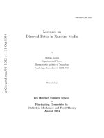
Hydrodynamic pressures on large lock structures

Hydrodynamic pressure on a lock gate

30
25
20

z [m]

Graduation committee:
prof. drs. ir. J.K. Vrijling
prof. dr. A.V. Metrikine
ir. W.F. Molenaar
ir. J. Manie
ir. P. Carree

15
10
5
0
-5

0

5

10

15

20

Re p [kPa]

Author
Student ID

:
:

Marco Versluis
1213393

Date

:

April 2010

1a

1b

1c

1d

25

Hydrodynamic pressures on large lock structures

Master of Science thesis
for acquisition of the degree
Master of Science in Civil Engineering
at Delft University of Technology

by
Marco Versluis
April 2010

Graduation committee:
prof. drs. ir. J.K. Vrijling (chairman)
Section of Hydraulic Engineering, Faculty of Civil Engineering and Geosciences, Delft University of Technology
prof. dr. A.V. Metrikine
Section of Structural Mechanics, Faculty of Civil Engineering and Geosciences, Delft University of Technology
ir. W.F. Molenaar
Section of Hydraulic Engineering, Faculty of Civil Engineering and Geosciences, Delft University of Technology
ir. J. Manie
Software Development Engineer, TNO DIANA
ir. P. Carree
Senior Structural Engineer, Witteveen+Bos Consulting Engineers



Hydrodynamic pressures on large lock structures

Preface
This thesis marks the end of my study Civil Engineering at Delft University of Technology at the department of

Hydraulic Engineering, faculty of Civil Engineering and Geosciences. This research project has been performed
in cooperation the engineering company Witteveen+Bos. Witteveen+Bos participated as subcontractor in the
tender design of the Panama Canal Third Set of Locks Project. The Panama isthmus is an area prone to
earthquakes and therefore seismic loading is an important aspect in the design of the new Post-Panamax locks.
Based on this project I chose the subject of my thesis: hydrodynamic pressure on large lock structures as a result
of earthquakes. The project also serves as a case study.
I would like to thank my supervisors: prof. drs. ir. J.K. Vrijling, prof. dr. A.V. Metrikine and ir. W.F. Molenaar
from the faculty, ir. J. Manie from TNO DIANA and ir. P. Carree from Witteveen+Bos for their guidance and
feedback.
Special thanks to my family who have always supported me.
Marco Versluis
Rotterdam, April 2010

v


Hydrodynamic pressures on large lock structures

vi


Hydrodynamic pressures on large lock structures

Abstract
When a navigation lock, dam, or any other structure with water is subjected to an earthquake, one of the dynamic
loads will be hydrodynamic pressure. This is the pressure exerted by the fluid on the structure as a result of the
different behavior in motion of solid and fluid. To determine this pressure there are several methods available
which focus mainly on large dams or fluid storage containers. The hydrodynamic behavior of these types of
structures is different and these methods may or may not be applicable for navigation locks. Therefore an
analysis is made to determine the factors that contribute to the hydrodynamic pressure distribution on large lock

structures.
As a case study the Third Set of Locks Project of the Panama Canal is used. This expansion project ensures that
the Panama Canal can process larger ships than the current Panamax class of ships, which dimensions are
limited by the existing locks. Therefore larger locks are required which will operate next to the existing locks.
The new locks are planned to be operational in 2014-2015. The Panama region is prone to earthquakes which
could result in large hydrodynamic pressures on the locks.
For the evaluation of hydrodynamic pressures on the gates and walls of large lock structures, two analytical (1D
and 2D) and one 2D finite-element model are made. These models are based on linear theory. Three main
aspects that contribute to hydrodynamic pressure are treated in detail:
• Lock dimensions and water levels;
• The effect of surface waves on the hydrodynamic pressure distribution;
• The stiffness of the structure.
In terms of dimensions, one of the main differences between lock chambers and large dams is the length of the
chamber or reservoir. The length of the chamber affects the hydrodynamic pressures in two ways: it limits the
impulsive (added mass) pressures but causes additional convective pressures due to sloshing. In general, the
effect of the chamber length on the magnitude of the hydrodynamic pressure is however limited. Only in the case
of a length over water depth ratio of 4 or smaller, there is a reduction of the pressure. For length over depth ratio
higher than 4, results are identical. This means only the water close to the gate or wall reacts and that for large
length the two boundaries can be treated individually. This is in agreement with the concept of added mass,
which assumes a body of water moving with a wall. A phase difference between two boundaries has therefore
almost no effect. Note that this can change for higher excitation frequencies.
The second way the chamber length influences the hydrodynamic pressure is a result of sloshing, which cannot
occur in a semi-infinite environment. Although for the large lock chambers many sloshing frequencies can be
found, in reality it takes too long for surface waves to cross the chamber to start the sloshing phenomenon. By
that time the earthquake is already over. In case of a very small length also little to no sloshing effects are to be
expected. If linear surface waves are neglected in the evaluation, the sloshing phenomenon cannot be identified.
Given the fact that neglecting surface waves greatly simplifies the analysis and has almost no outcome on the
solution; it can be concluded that this assumption of neglecting surface waves is also valid for navigation locks.
This conclusion is bases on the results obtained by the two analytical models. In the finite element results, no
sloshing frequencies could be identified.

Another difference in dimensions between navigation locks and large, high-head dams is the water depth. If
compressibility of water is taken into account, the impounded water has eigenfrequencies for hydrodynamic
pressure. These eigenfrequencies are inversely proportional to the water depth, meaning that the fundamental
eigenfrequency is lower for larger water depth. The water depth inside a navigation lock is directly related to the
draught of the design vessel and is therefore much smaller than in the case of a high-head dam. For the
maximum water depth of the Post-Panamax locks, around 30 m, the fundamental eigenfrequency related to
compressibility is larger than the frequencies at which the most energy of an earthquake is distributed. For
excitation frequencies below this fundamental eigenfrequency, the amplitude of hydrodynamic pressure is almost
independent of the excitation frequency. Also, the assumption of incompressible water gives in this situation
similar results. Therefore, the limited water depth in navigation locks means that in practice the hydrodynamic
pressure is constant for the considered frequencies and the assumption of incompressible water is valid. The
pressure distribution along the face of a gate/wall remains parabolic in this frequency range. For higher
excitation frequencies, above the fundamental eigenfrequency related to compressibility, the pressure
distribution is no longer parabolic, but sinusoidal and the assumptions are not valid anymore.

vii


Hydrodynamic pressures on large lock structures

The above conclusions are based on the assumption of rigid gates and/or walls. With the aid of the 2D finite
element model rigid gates were replaced with gates with a certain bending stiffness. The bending stiffness of the
used gates and the position of the supports are estimated, but the result in amplitude is significantly different.
The maximum pressure along the face is no longer at the bottom of the gate, but higher up. Although this applies
to a single case, it shows that the assumption of rigid gates/walls has to be applied with care.
Based on the findings of this thesis the following recommendations can be made:
• The performed analyses are performed in a 2D environment, with direction of earthquake loading
perpendicular to a lock gate. Other source-to-site directions and the effects of the side walls are not
incorporated. The reduced amount of water that can react in both cases should lead to a reduction of the
hydrodynamic pressure compared to the case in a 2D environment. This is shown by effect of the length of

the chamber. The presence of a ship inside the lock chamber during an earthquake might also reduce the
hydrodynamic pressure on the structure as the amount of water inside the chamber is less due to the
displacement of the vessel. With a 3D analysis these effects can be investigated.
• Surface waves and effects like sloshing have little to no influence on the total pressure distribution.
Therefore the assumption that the pressure at the water surface is equal to zero is also valid for navigation
locks and recommended for practical design.
• The stiffness of the structure is not incorporated in the solution of the 2D analytical model or the
Westergaard and Housner solution. An adaption of the 2D finite element model showed that the stiffness
and support system of a lock gate do change the loading on the lock gate. Therefore it is recommended that
a preliminary analysis is made to investigate if a closed or (semi-)opened gate, or the chamber itself can be
treated as rigid. If not, the stiffness of the structure should be incorporated in the evaluation, as it can result
in a significant in- or decrease of the hydrodynamic loading.
• Not only the horizontal component of an earthquake, but also the vertical component causes hydrodynamic
pressures on walls. This aspect is not treated in this thesis, but would be an interesting element to include in
future studies. The vertical component is in general smaller than the horizontal component.
• Analyses made in this thesis are done in the frequency domain; a time domain analysis is not performed but
gives more insight in the hydrodynamic pressures during the event of an earthquake.
• The existing analytical methods by Westergaard or Housner give adequate accuracy and can by used in early
design stages. The loads can be evaluated by means of pressure or the concept of added mass. An estimate
for the accuracy can be obtained by comparing a spectrum with the fundamental eigenfrequency for the
maximum design water level. For later design stages the use of advanced methods should be used to
determine the hydrodynamic pressures and consequently the response of the structure. As stated before, the
analytical Westergaard and Housner approaches do not incorporate the frequency-dependent motion of the
structure, but assume a rigid behavior. A finite element analysis using fluid-structure interaction can
incorporate these effects and will therefore give in general a more accurate result. That this is not always the
case followed from the finite element model used in this thesis, which failed to identify possible sloshing
frequencies.

viii

Hydrodynamic pressures on large lock structures

Table of contents
PREFACE ....................................................................................................................................................................................................................... V
ABSTRACT ................................................................................................................................................................................................................. VII
TABLE OF CONTENTS...............................................................................................................................................................................................IX
LIST OF FIGURES .......................................................................................................................................................................................................XI
LIST OF TABLES ....................................................................................................................................................................................................... XII
LIST OF SYMBOLS ..................................................................................................................................................................................................XIII
1.

INTRODUCTION .................................................................................................................................................................................................1
1.1.
1.2.

2.

PROJECT BACKGROUND ................................................................................................................................................................................3
2.1.
2.2.
2.3.
2.4.
2.4.1.
2.4.2.
2.4.3.

3.

OBJECTIVES OF THESIS ...................................................................................................................................................................................1

LAYOUT OF THESIS ........................................................................................................................................................................................1

HISTORY OF THE PANAMA CANAL .................................................................................................................................................................3
CURRENT LAYOUT OF THE PANAMA CANAL ...................................................................................................................................................3
THIRD SET OF LOCKS EXPANSION PROJECT ...................................................................................................................................................4
PROPOSED DESIGN .........................................................................................................................................................................................5
General and chamber dimensions .......................................................................................................................................................5
Lock heads..........................................................................................................................................................................................6
Lock gates ..........................................................................................................................................................................................8

EARTHQUAKES..................................................................................................................................................................................................9
3.1.
INTRODUCTION ..............................................................................................................................................................................................9
3.2.
TYPES OF EARTHQUAKES ...............................................................................................................................................................................9
3.3.
SEISMIC WAVES ...........................................................................................................................................................................................10
3.3.1.
P-waves ............................................................................................................................................................................................10
3.3.2.
S-waves ............................................................................................................................................................................................11
3.3.3.
Rayleigh waves.................................................................................................................................................................................11
3.3.4.
Love-waves ......................................................................................................................................................................................11

4.

COMMONLY USED PROCEDURES FOR (HYDRO)DYNAMIC ANALYSES ..........................................................................................13
4.1.

4.2.
4.3.
4.4.
4.5.
4.6.
4.7.
4.7.1.
4.7.2.
4.7.3.

5.

INTRODUCTION ............................................................................................................................................................................................13
QUASI-STATIC (SEISMIC COEFFICIENT METHOD )...........................................................................................................................................13
RESPONSE SPECTRUM ANALYSIS ..................................................................................................................................................................14
TIME-HISTORY ANALYSIS .............................................................................................................................................................................14
HYBRID FREQUENCY T IME DOMAIN ANALYSIS ............................................................................................................................................15
A BRIEF INTRODUCTION TO THE FINITE E LEMENT METHOD .........................................................................................................................15
HYDRODYNAMIC PRESSURES .......................................................................................................................................................................16
Hydrodynamic pressure according to Westergaard ...........................................................................................................................16
Hydrodynamic pressure according to Housner .................................................................................................................................18
Transformation to added mass ..........................................................................................................................................................21

SITE CONDITIONS AND PRELIMINARY ASSESSMENT..........................................................................................................................23
5.1.
BOUNDARY CONDITIONS ..............................................................................................................................................................................23
5.1.1.
Seismic conditions............................................................................................................................................................................23
5.1.2.
Soil and rock properties ....................................................................................................................................................................23

5.2.
PRELIMINARY ASSESSMENT: THE WESTERGAARD AND HOUSNER FORMULAS APPLIED .................................................................................23
5.3.
HOUSNER'S MATHEMATICAL MODEL ............................................................................................................................................................25
5.3.1.
Introduction to Housner's model .......................................................................................................................................................25
5.3.2.
Response spectrum approach ............................................................................................................................................................25
5.3.3.
SDOF approach ................................................................................................................................................................................26
5.3.4.
Conclusions Housner's model ...........................................................................................................................................................27

6.

ONE-DIMENSION MODEL FOR WAVE INTERACTION ..........................................................................................................................29
6.1.
6.2.
6.3.
6.4.
6.5.
6.6.
6.7.
6.8.
6.8.1.
6.8.2.
6.9.
6.10.

INTRODUCTION 1D MODEL...........................................................................................................................................................................29

STRATEGY ...................................................................................................................................................................................................29
THE 1D MODEL OF A LOCK HEAD .................................................................................................................................................................30
EQUATIONS OF MOTION ...............................................................................................................................................................................34
STEADY-STATE SOLUTIONS ..........................................................................................................................................................................34
BOUNDARY CONDITIONS ..............................................................................................................................................................................35
APPLYING BOUNDARY AND INTERFACE CONDITIONS ....................................................................................................................................36
SOLUTIONS IN THE FREQUENCY DOMAIN ......................................................................................................................................................36
Solution to the wave equation only...................................................................................................................................................36
Response to inertia force...................................................................................................................................................................37
NUMERIC VALUES ........................................................................................................................................................................................37
CONCLUSIONS 1D MODEL FOR WAVE INTERACTION .....................................................................................................................................39

ix


Hydrodynamic pressures on large lock structures

7.

TWO-DIMENSIONAL MODEL FOR HYDRODYNAMIC PRESSURE ......................................................................................................43
7.1.
INTRODUCTION 2D MODEL...........................................................................................................................................................................43
7.2.
STRATEGY ...................................................................................................................................................................................................43
7.3.
2D MODEL AND BOUNDARY CONDITIONS .....................................................................................................................................................44
7.4.
EIGENFREQUENCIES OF THE SYSTEM ............................................................................................................................................................45
7.5.
STEADY-STATE SOLUTION ............................................................................................................................................................................46

7.6.
SOLUTION IN THE FREQUENCY DOMAIN ........................................................................................................................................................46
7.7.
NUMERIC VALUES ........................................................................................................................................................................................47
7.8.
FREQUENCY DOMAIN RESULTS OF THE 2D MODEL........................................................................................................................................47
7.8.1.
Eigenfrequencies ..............................................................................................................................................................................47
7.8.2.
Hydrodynamic pressure at bottom of gate (situation long lock chamber) .........................................................................................48
7.8.3.
Hydrodynamic pressure at top of gate (situation long lock chamber) ...............................................................................................48
7.8.4.
Hydrodynamic pressure at bottom of gate (situation shorter intermediate chamber).........................................................................50
7.8.5.
Hydrodynamic pressure at top of gate (situation shorter intermediate chamber)...............................................................................50
7.8.6.
Hydrodynamic pressure along the face of the gate (situation long lock chamber).............................................................................51
7.8.7.
Hydrodynamic pressure along the face of the gate (situation shorter intermediate chamber) ............................................................53
7.8.8.
The effect of surface waves ..............................................................................................................................................................55
7.8.9.
Length and depth of lock chamber....................................................................................................................................................55
7.9.
COMPARISON WITH WESTERGAARD'S RESULTS ............................................................................................................................................56
7.10.
CONCLUSIONS 2D MODEL FOR HYDRODYNAMIC PRESSURE ..........................................................................................................................57
7.10.1.
Solution ............................................................................................................................................................................................57

7.10.2.
Resonance effects .............................................................................................................................................................................57
7.10.3.
Effect of surface waves.....................................................................................................................................................................58
7.10.4.
Phase difference and chamber length................................................................................................................................................58
7.10.5.
Compressibility effects .....................................................................................................................................................................58

8.

TWO-DIMENSIONAL MODEL FOR FLUID-STRUCTURE INTERACTION...........................................................................................59
8.1.
8.2.
8.3.
8.3.1.
8.3.2.
8.3.3.
8.4.
8.4.1.
8.4.2.
8.4.3.
8.4.4.
8.4.5.
8.4.6.
8.4.7.
8.5.
8.5.1.
8.5.2.
8.5.3.

8.5.4.

9.

INTRODUCTION ............................................................................................................................................................................................59
STRATEGY ...................................................................................................................................................................................................60
PREPROCESSING: ELEMENT TYPES AND NUMERICAL VALUES ........................................................................................................................60
Introduction ......................................................................................................................................................................................60
Element types ...................................................................................................................................................................................61
Numerical values ..............................................................................................................................................................................62
RESULTS IN THE FREQUENCY DOMAIN ..........................................................................................................................................................63
Introduction ......................................................................................................................................................................................63
Hydrodynamic pressure at bottom of gate (situation long lock chamber) .........................................................................................63
Hydrodynamic pressure at bottom of gate (situation shorter intermediate chamber).........................................................................67
Hydrodynamic pressure along the face of the gate (situation long lock chamber).............................................................................69
Hydrodynamic pressure along the face of the gate (situation shorter intermediate chamber) ............................................................74
Effect of the stiffness of the gates.....................................................................................................................................................78
Semi-infinite chamber ......................................................................................................................................................................81
CONCLUSIONS 2D MODEL FOR FLUID -STRUCTURE INTERACTION ..................................................................................................................84
Solution ............................................................................................................................................................................................84
Comparison of results with the 2D analytical model.........................................................................................................................84
Compressibility effects .....................................................................................................................................................................84
Special models..................................................................................................................................................................................84

CONCLUSIONS AND RECOMMENDATIONS .............................................................................................................................................87
9.1.
9.2.

CONCLUSIONS .............................................................................................................................................................................................87
RECOMMENDATIONS ....................................................................................................................................................................................87

REFERENCES ..............................................................................................................................................................................................................89
APPENDIX A: GEOLOGICAL MAP OF THE ISTHMUS OF PANAMA ............................................................................................................ A.1
A.1

EXPLANATION ........................................................................................................................................................................................... A.1

APPENDIX B: DERIVATIONS AND DETAILED CALCULATIONS................................................................................................................. B.1
A.1

B.1
B.2
B.3
B.3.1
B.3.2
B.3.3
B.4
B.5
B.5.1
B.5.2
B.6
B.7
B.7.1
B.7.2

THE WESTERGAARD AND CHOPRA SOLUTIONS IN DETAIL ......................................................................................................................... B.1
SOLVING HOUSNER 'S SDOF MODEL .......................................................................................................................................................... B.2
DERIVATION OF THE 1D SHALLOW WATER EQUATIONS .............................................................................................................................. B.3
Introduction .................................................................................................................................................................................... B.3
Continuity equation ........................................................................................................................................................................ B.3

Momentum balance equation .......................................................................................................................................................... B.4
DERIVATION OF THE 1D WAVE EQUATION .................................................................................................................................................. B.7
SOLVING THE 1D MODEL UNDER WAVE LOADING ....................................................................................................................................... B.7
Fluid boundaries ............................................................................................................................................................................. B.7
Gates A & B ................................................................................................................................................................................... B.8
DERIVATION OF THE 2D WAVE EQUATION .................................................................................................................................................. B.8
SOLVING THE 2D MODEL FOR HYDRODYNAMIC PRESSURE ......................................................................................................................... B.9
Homogenous solution ..................................................................................................................................................................... B.9
Steady-state solution..................................................................................................................................................................... B.10
A.1

APPENDIX C: THE FINITE ELEMENT PROGRAM DIANA ............................................................................................................................. C.1
B.1

C.1
C.2

WORKFLOW IN DIANA ............................................................................................................................................................................ C.1
DIANA BROCHURE AND BACKGROUND THEORY FSI ................................................................................................................................. C.1
B.1

x


Hydrodynamic pressures on large lock structures

List of figures
FIGURE 2.1 CROSS-SECTION OF THE PANAMA CANAL
FIGURE 2.2 LAYOUT OF THE PANAMA CANAL
FIGURE 2.3 CONCEPTUAL ISOMETRIC VIEW OF THE NEW LOCKS COMPLEX (ADAPTED FROM [PANAMA CANAL AUTHORITY, 2006])

FIGURE 2.4 AERIAL VIEW OF THE CONSTRUCTION SITES OF THE NEW LOCKS, INDICATED BY RED ARROW (ADAPTED FROM [PANAMA CANAL AUTHORITY, 2006])
FIGURE 2.5 COMPARISON BETWEEN VESSEL AND LOCK DIMENSIONS OF THE NEW AND EXISTING LOCKS (ADAPTED FROM [PAYER, 2005]
FIGURE 2.6 ARTIST IMPRESSION OF THE POST-PANAMAX LOCKS, PACIFIC SIDE
FIGURE 2.7 CROSS-SECTION WITH MAIN DIMENSIONS OF THE L-WALL TYPE LOCK CHAMBER
FIGURE 2.8 ARTIST IMPRESSION OF A LOCK HEAD UNDER CONSTRUCTION
FIGURE 2.9.A TOP VIEW WITH STRUCTURAL COMPONENTS LOCK HEADS (SOURCE: WITTEVEEN+BOS)
FIGURE 2.9.B LONGITUDINAL CROSS-SECTION WITH STRUCTURAL COMPONENTS LOCK HEADS
FIGURE 2.9.C CROSS-SECTION OF A LOCK HEAD WITH THE STRUCTURAL COMPONENTS
FIGURE 2.10 SKETCH CROSS-SECTION OF LOCK GATE
FIGURE 3.1 TECTONIC PLATES IN THE REGION
FIGURE 3.2 SUBDUCTION ZONE AT BOUNDARY OF OCEANIC AND CONTINENTAL PLATE (SOURCE: ROBERT SIMMON, NASA GSFC)
FIGURE 3.3 TYPES OF FAULTS
FIGURE 3.4 MAJOR FAULT LINES IN THE CANAL ZONE (ADAPTED FROM U.S. (SOURCE: U.S. GEOLOGICAL SURVEY) GEOLOGICAL SURVEY, 1998])
FIGURE 3.5 TYPES OF SEISMIC WAVES
FIGURE 4.1 ACCELERATION TIME HISTORY OR ACCELEROGRAM
FIGURE 4.2 PROCEDURE FOR MAKING
FIGURE 4.3 HORIZONTAL RESPONSE SPECTRA FOR A DAMPING RATIO OF 5%
FIGURE 4.4 DISCRETIZATION OF A DOMAIN BY MEANS OF ELEMENTS
FIGURE 4.5 INTERPOLATION BY SHAPE FUNCTIONS
FIGURE 4.6 HYDRODYNAMIC PRESSURE DISTRIBUTION FOR THE ORIGINAL (LEFT) AND SIMPLIFIED PARABOLA (RIGHT) WESTERGAARD SOLUTIONS (ADAPTED FROM [WESTERGAARD, 1933])
FIGURE 4.7 CORRECTION FACTOR ON THE WESTERGAARD FORMULA IN CASE OF SHORT RESERVOIR
FIGURE 4.8 HYPERBOLIC FUNCTIONS
FIGURE 4.9 HOUSNER'S MATHEMATICAL MODEL FOR IMPULSIVE AND CONVECTIVE HYDRODYNAMIC FORCES (ADAPTED FROM [USACE, EM 1110-2-6051])
FIGURE 4.10 HYDRODYNAMIC PRESSURE DISTRIBUTION IN THE CASE OF D/L > 1.6 ACCORDING TO HOUSNER
FIGURE 5.1 COMPARISON OF HYDRODYNAMIC PRESSURE ACCORDING TO THE WESTERGAARD AND HOUSNER FORMULAS
FIGURE 5.2 SDOF MASS-SPRING SYSTEM FOR CALCULATING SLOSHING FORCE
FIGURE 5.3 DIMENSIONLESS AMPLITUDE-FREQUENCY RESPONSE FUNCTION FOR HOUSNER'S SDOF MODEL
FIGURE 6.1 SKETCH CROSS-SECTION OF AN ARBITRARY LOCK HEAD
FIGURE 6.2 1D MODEL OF A LOCK HEAD
FIGURE 6.3 HYDROSTATIC PRESSURES AND REFERENCE LEVEL

FIGURE 6.4 SDOF MASS-SPRING SYSTEM
FIGURE 6.5 PROCEDURE FOR FINDING SOLUTION IN THE FREQUENCY AND TIME DOMAIN (ADAPTED FROM [KRAMER, 1996])
FIGURE 6.6 SITUATION AT INTERFACE GATE-WATER WHEN GATE MOVES IN POSITIVE X-DIRECTION
FIGURE 6.7 MODES SHAPE FOR THE FIRST THREE EIGENFREQUENCIES
FIGURE 6.8 THE FREQUENCY RESPONSE OF LOCK GATE A UNDER DIFFERENT COMPONENTS OF LOADING, INCLUDING DETAIL
FIGURE 6.9 THE FREQUENCY RESPONSE OF LOCK GATE B UNDER DIFFERENT COMPONENTS OF LOADING, INCLUDING DETAIL
FIGURE 7.1 2D MODEL FOR HYDRODYNAMIC PRESSURES, WITH BOUNDARY CONDITIONS
FIGURE 7.2 HYDRODYNAMIC PRESSURES: WITH (TOP) AND WITHOUT (BOTTOM) PHASE DIFFERENCE BETWEEN THE GATES
FIGURE 7.3 HYDRODYNAMIC PRESSURES: WITH (TOP), WITHOUT (CENTER) PHASE DIFFERENCE BETWEEN THE GATES AND DETAIL (BOTTOM)
FIGURE 7.4 HYDRODYNAMIC PRESSURES, WITH (TOP) AND WITHOUT (BOTTOM) A PHASE DIFFERENCE BETWEEN THE GATES
FIGURE 7.5 HYDRODYNAMIC PRESSURES, WITH (TOP) AND WITHOUT (BOTTOM) A PHASE DIFFERENCE BETWEEN THE GATES
FIGURE 7.6 HYDRODYNAMIC PRESSURE DISTRIBUTION AT ΩE ≈ 0.63 RAD/S (0.1 HZ)
FIGURE 7.7 HYDRODYNAMIC PRESSURE DISTRIBUTION AT ΩE ≈ 2.51 RAD/S (0.4 HZ)
FIGURE 7.8 HYDRODYNAMIC PRESSURE DISTRIBUTION AT ΩE ≈ 6.28 RAD/S (1 HZ)
FIGURE 7.9 HYDRODYNAMIC PRESSURE DISTRIBUTION AT ΩE ≈ 37.70 RAD/S (6 HZ)
FIGURE 7.10 HYDRODYNAMIC PRESSURE DISTRIBUTION AT ΩE ≈ 0.63 RAD/S (0.1 HZ)
FIGURE 7.11 HYDRODYNAMIC PRESSURE DISTRIBUTION AT ΩE ≈ 2.51 RAD/S (0.4 HZ)
FIGURE 7.12 HYDRODYNAMIC PRESSURE DISTRIBUTION AT ΩE ≈ 6.28 RAD/S (1 HZ)
FIGURE 7.13 HYDRODYNAMIC PRESSURE DISTRIBUTION AT ΩE ≈ 37.70 RAD/S (6 HZ)
FIGURE 7.14 HYDRODYNAMIC PRESSURES IN CASE OF A ZERO PRESSURE BOUNDARY CONDITION
FIGURE 7.15 MAXIMUM HYDRODYNAMIC PRESSURE AT THE BOTTOM OF A GATE FOR DIFFERENT CHAMBER LENGTHS AT 1 HZ
FIGURE 7.16 THE WESTERGAARD SOLUTION IN COMPARISON WITH EQUATION (7.18), WITH DETAIL FOR LOW FREQUENCIES
FIGURE 8.1 2D MODEL FOR FEM ANALYSIS WITH RIGID GATES
FIGURE 8.2 2D MODEL FOR FEM ANALYSIS WITH FLEXIBLE GATES
FIGURE 8.3 2D MODEL FOR SEMI-INFINITE FEM ANALYSIS WITH RIGID GATE
FIGURE 8.4 FEM MESH FOR MODEL 2D
FIGURE 8.5 THE BCL63S FLUID-STRUCTURE ELEMENT, LINE, 3+3 NODES (ADAPTED FROM [TNO DIANA, 2008])
FIGURE 8.6 NODAL CONNECTIVITY FOR 2D FLUID-STRUCTURE INTERACTION (ADAPTED FROM [TNO DIANA, 2008])
FIGURE 8.7A HYDRODYNAMIC PRESSURES FOR CASE 1A
FIGURE 8.7B HYDRODYNAMIC PRESSURES FOR CASE 1B

FIGURE 8.7C HYDRODYNAMIC PRESSURES FOR CASE 1C (BOTTOM AND TOP LEVEL OF GATE)
FIGURE 8.7D HYDRODYNAMIC PRESSURES FOR CASE 1D (BOTTOM AND TOP LEVEL OF GATE)
FIGURE 8.8A HYDRODYNAMIC PRESSURES FOR CASE 2A
FIGURE 8.8B HYDRODYNAMIC PRESSURES FOR CASE 2B
FIGURE 8.8C HYDRODYNAMIC PRESSURES FOR CASE 2C (BOTTOM AND TOP LEVEL OF GATE)
FIGURE 8.8D HYDRODYNAMIC PRESSURES FOR CASE 2D (BOTTOM AND TOP LEVEL OF GATE)
FIGURE 8.9 HYDRODYNAMIC PRESSURE DISTRIBUTION AT ΩE = 2Π RAD/S (1.00 HZ)
FIGURE 8.10 HYDRODYNAMIC PRESSURE DISTRIBUTION AT ΩE = Ω1/2 ≈ 37.70 RAD/S (6.00 HZ)
FIGURE 8.11 HYDRODYNAMIC PRESSURE DISTRIBUTION AT ΩE < Ω1 ≈ 75.40 RAD/S (12.00 HZ)
FIGURE 8.12 HYDRODYNAMIC PRESSURE DISTRIBUTION AT ΩE > Ω1 ≈ 76.97 RAD/S (12.25 HZ)
FIGURE 8.13 HYDRODYNAMIC PRESSURE DISTRIBUTION AT ΩE = (Ω1+Ω2)/2 ≈ 152.37 RAD/S (24.25 HZ)
FIGURE 8.14 HYDRODYNAMIC PRESSURE DISTRIBUTION AT ΩE < Ω2 ≈ 227.77 RAD/S (36.25 HZ)
FIGURE 8.15 HYDRODYNAMIC PRESSURE DISTRIBUTION AT ΩE > Ω2 ≈ 229.34 RAD/S (36.50 HZ)
FIGURE 8.16 HYDRODYNAMIC PRESSURE DISTRIBUTION AT ΩE = 2Π ≈ 6.28 RAD/S (1.00 HZ)
FIGURE 8.17 HYDRODYNAMIC PRESSURE DISTRIBUTION AT ΩE = Ω1/2 ≈ 37.70 RAD/S (6.00 HZ)
FIGURE 8.18 HYDRODYNAMIC PRESSURE DISTRIBUTION AT ΩE < Ω1 ≈ 75.40 RAD/S (12.00 HZ)
FIGURE 8.19 HYDRODYNAMIC PRESSURE DISTRIBUTION AT ΩE > Ω1 ≈ 76.97 RAD/S (12.25 HZ)
FIGURE 8.20 HYDRODYNAMIC PRESSURE DISTRIBUTION AT ΩE = (Ω1+Ω2)/2 ≈ 152.37 RAD/S (24.25 HZ)
FIGURE 8.21 HYDRODYNAMIC PRESSURE DISTRIBUTION AT ΩE < Ω2 ≈ 227.77 RAD/S (36.25 HZ)
FIGURE 8.22 HYDRODYNAMIC PRESSURE DISTRIBUTION AT ΩE > Ω2 ≈ 229.34 RAD/S (36.50 HZ)
FIGURE 8.23 HYDRODYNAMIC PRESSURES (CASE FLEXIBLE GATES, LONG LOCK CHAMBER): BOTTOM OF GATE (TOP), COMPARISON WITH CASE 1D (CENTER) AND TOP OF GATE (BOTTOM)
FIGURE 8.24 HYDRODYNAMIC PRESSURES (CASE FLEXIBLE GATES, SHORTER INTERMEDIATE CHAMBER): BOTTOM OF GATE (TOP), COMPARISON WITH CASE 2D (CENTER) AND TOP OF GATE (BOTTOM)
FIGURE 8.25 HYDRODYNAMIC PRESSURE DISTRIBUTION IN CASE OF FLEXIBLE GATES: SITUATION LONG LOCK CHAMBER (TOP) AND SITUATION SHORTER INTERMEDIATE CHAMBER (BOTTOM)
FIGURE 8.26 HYDRODYNAMIC PRESSURES (CASE SEMI-INFINITE CHAMBER): BOTTOM OF GATE INCLUDING COMPARISON WITH CASE 1D (TOP) AND TOP OF GATE (BOTTOM)
FIGURE 8.27 HYDRODYNAMIC PRESSURE DISTRIBUTION IN CASE OF SEMI-INFINITE CHAMBER: REAL (TOP) AND IMAGINARY PARTS (BOTTOM)
FIGURE B.1 HYDRODYNAMIC PRESSURES ACCORDING TO CHOPRA
FIGURE B.2 CONTROL AREA FOR DERIVATION OF THE CONTINUITY EQUATION
FIGURE B.3 CONTROL VOLUME FOR DERIVATION OF THE MOMENTUM BALANCE EQUATION
FIGURE B.4 CONTROL AREA FOR DERIVATION OF THE MOMENTUM BALANCE EQUATION

3
4
4
4
5
6
6
6
7
7
7
8
9
9
10
10
10
13
14
14
15
16
17
18
19
19
20
24
26
27

30
30
31
32
33
34
36
40
41
45
48
49
50
51
52
52
52
53
53
54
54
54
55
56
57
59
60
60
61
62

62
64
64
65
66
67
67
68
69
70
71
71
72
72
73
73
74
75
75
76
76
77
77
79
80
81
83
83
B.2
B.4

B.4
B.6

xi


Hydrodynamic pressures on large lock structures

List of tables
TABLE 5.1 DIFFERENCES BETWEEN A LEVEL 1 AND LEVEL 2 EARTHQUAKE AS DEFINED IN THE PROGRAM OF REQUIREMENTS ...........................................................................................................................23
TABLE 5.2 ROCK MASS PROPERTIES OF BEDROCK PRESENT AT THE PACIFIC AND ATLANTIC SITES.....................................................................................................................................................................23
TABLE 5.3 ADDED MASS COMPARISON FOR LONG RESERVOIRS OR LOCK CHAMBERS .........................................................................................................................................................................................25
TABLE 5.4 RESULTS FOR HOUSNER'S SDOF MODEL (1ST MODE ONLY)...............................................................................................................................................................................................................27
TABLE 7.1. A FIRST 25 EIGENFREQUENCIES FOR THE LONG LOCK CHAMBER .......................................................................................................................................................................................................47
TABLE 7.1. B FIRST 25 EIGENFREQUENCIES FOR THE SHORTER INTERMEDIATE CHAMBER ...................................................................................................................................................................................47
TABLE 7.2 SELECTED EXCITATION FREQUENCIES WITH CORRESPONDING FIGURES (SITUATION LONG LOCK CHAMBER) .....................................................................................................................................51
TABLE 7.3 SELECTED EXCITATION FREQUENCIES WITH CORRESPONDING FIGURES (SITUATION SHORTER INTERMEDIATE CHAMBER) .................................................................................................................53
TABLE 8.1 SELECTED EXCITATION FREQUENCIES WITH CORRESPONDING FIGURES (SITUATION LONG LOCK CHAMBER) .....................................................................................................................................70
TABLE 8.2 SELECTED EXCITATION FREQUENCIES WITH CORRESPONDING FIGURES (SITUATION LONG LOCK CHAMBER) .....................................................................................................................................74

xii


Hydrodynamic pressures on large lock structures

List of symbols
Not all symbols have been listed as some have only local meaning. A few symbols have more than one meaning.

English
Symbol

Description

SI unit

a

acceleration

[m/s2]

c

damping coefficient

[kg/s]

cp

celerity of pressure waves

[m/s]

cP

celerity of P-waves

[m/s]

cR

celerity of Rayleigh waves

[m/s]

cS

celerity of S-waves

[m/s]

cw

celerity of surface waves

[m/s]

Cn

constant taking in account compressibility of water in the Westergaard formula

[-]

d

constant water depth

[m]

E

fe

Young's modulus

[Pa]

harmonic excitation frequency

[Hz]

F1

force related to convective pressure (1st mode)

[N/m]

Fd

hydrostatic force

[N/m]

Fe

earthquake force

[N/m]

Fη
g

wave force

[N/m]

acceleration of gravity

[m/s2]

G

shear modulus

[Pa]

h

height on which hydrodynamic forces acts in Housner's model

[m]

h
Hˆ

total water depth

[m]

complex frequency response function for η

[m]

I

momentum

[N·s]

k

spring stiffness

[N/m]

k
kh

wavenumber

[m-1]

horizontal seismic coefficient

[-]
st

K1

spring stiffness related to convective pressure (1 mode) in Housner's model

[N/m]

K

bulk modulus

[Pa]

L
m

distance, (half) lock chamber length

[m]

mass

[kg/m]

mam

added mass

[kg/m]

M

P-wave modulus

[Pa]

xiii


Hydrodynamic pressures on large lock structures

M
M0

total water mass in chamber in Housner's model

[kg/m]

mass related to impulsive pressure in Housner's model

[kg/m]

M1

mass related to convective pressure (1st mode) in Housner's model

[kg/m]

Mw
p

moment magnitude

[-]

(hydrodynamic) pressure

[Pa]

Pˆ

complex frequency response function for p

[Pa]

PGA

peak ground acceleration

[m/s2]

Ra

acceleration response spectrum

[m/s2]

t

time variable

[s]

T

period

[s]

T1

fundamental eigenperiod

[s]

Te

harmonic excitation period

[s]

Tn

eigenperiod

[s]

Tr

return period

[s]

u

displacement

[m]

ue
x
y

earthquake excitation acceleration

[m/s2]

horizontal coordinate

[m]

vertical coordinate

[m]

z

vertical coordinate

[m]

Symbol

Description

SI unit

β
γ

correction factor on Westergaard's formula

[-]

specific weight

[N/m3]

ε
ζ
η

volumetric strain

[-]

damping ratio

[-]

surface wave amplitude

[m]

λ

ν
ρ

wavelength

[m]

Poisson's ratio

[-]

density

[kg/m3]

σ
υ
ϕ

stress

[Pa]

flow velocity

[m/s]

phase

[-]

ωe
ωn

(angular) harmonic excitation frequency

[rad/s]

(angular) natural frequency

[rad/s]

Greek

xiv


Hydrodynamic pressures on large lock structures

1. Introduction

1. Introduction
1.1.

Objectives of thesis

The objective of this thesis is to research the earthquake induced hydrodynamic pressure on a lock structure.
When a navigation lock is subjected to an earthquake, the structure itself and the water inside the chamber will
react differently. The different behavior causes a reaction load by the water on the lock structure. Besides an
always present hydrostatic pressure, an earthquake will exert an extra hydrodynamic pressure on the lock. The

magnitude of this hydrodynamic pressure depends on many aspects. The effect of each of these aspects on the
hydrodynamic pressure will be investigated by a series of models. The following aspects will be treated in detail:
• Lock dimensions and water levels
The amount of water has a large influence on the pressure distribution. In general the principle of "the more
water, the more pressure", holds. But the way the water reacts inside a lock chamber is different than e.g.
behind a dam. Seismic waves, originating from the source of earthquake, travel towards the structure with a
certain velocity. This means that for large structure the acceleration at a certain point of time is not constant
for the whole structure. For navigation locks this means that one side vibrates different from the other side
because of this phase lag. The dimensions of a lock chamber (chamber length, width and water depth) are
different than dams or fluid storage container, which results in a possible different behavior.
• The effect of surface waves on the hydrodynamic pressure distribution
When a contained body of water – with a free surface – is set in motion, waves at the surface will be
generated. These waves influence the hydrodynamic pressure below and at the water surface. If the wave
pressure is small enough compared with the total pressure, the effect can be neglected which simplifies a
computation, which is done with most methods to calculate hydrodynamic pressures. The conditions under
which such an assumption is valid, or not, will be investigated.
• Stiffness of the structure
The hydrodynamic pressure on a structure depends on the stiffness of that structure. A rigid wall behaves
different than a flexible wall. Because the hydrodynamic pressure is a reaction load, it is influenced by the
stiffness.
There are many methods available for the calculation of hydrodynamic pressure: from relative simple analytical
formulas to full computer-based analyses. The analytical formula's are based on large dams or fluid storage
containers, which each have a different scale than navigation locks and are affected differently by the above
mentioned aspects. The available analytical methods will be reviewed for the application to navigation locks.
Besides the previously mentioned aspects, other factors contribute to the hydrodynamic loading on a lock
structure. These include the e.g. the presence of ship inside a lock, the opening and closing of gates and the
direction of the source of the earthquake. Models in this thesis are based upon a closed lock gates or walls which
are loaded perpendicular and have no ships inside the lock chambers. The models focus on large lock structures,
the Third Set of Locks project of the Panama Canal is used as a case example for dimensions. A total of three
models will be discussed:

1. An analytical 1D model of a lock head to investigate the effect of surface waves;
2. An analytical 2D model of a single lock chamber which includes all of the above mentioned aspects, except
the stiffness of the lock (gates);
3. A computer-based model based on the analytical 2D model, but with the ability to include e.g. the stiffness
of the lock gates.
With these three models the hydrodynamic pressure on a lock structure will be investigated. The response of the
structure is not treated in detail.

1.2.

Layout of thesis

More information about the history and the expansion project of the Panama Canal, which is used as a case study,
can be found in the next chapter. Background theory about earthquakes and (hydro)dynamic analyses is treated in
chapters 3 and 4. In chapter 5 the site conditions specific for the Panama Canal are listed and a preliminary
assessment of the magnitude of hydrodynamic pressure is made. Further chapters (6, 7 and 8) treat the abovementioned three models.

1


Hydrodynamic pressures on large lock structures

1. Introduction

2


Hydrodynamic pressures on large lock structures

2. Project background

2. Project background
2.1.

History of the Panama Canal

Plans for the construction of a canal between the Atlantic and Pacific Oceans date back to the late 16th century.
The strategic situation of the Panama Isthmus led to the construction of the Panama Railway from 1850 to 1855,
which was the first fast and less risky alternative for the trading routes used prior to the 19th century to transport
goods between the two oceans.
After the success of Suez Canal in 1869 the French started to work on the Panama Canal in 1880, but
construction was abandoned in 1893 due to several problems. The French plan was to build a canal on sea level,
which proved to be very difficult. Combined with deceases, landslides and insufficient knowledge about the
geology and hydrology of the country, the attempt cost the lives of about 21,900 workers. After the failed attempt
by the French, the Americans continued the work in 1904. Because Panama was under Colombian control, the
United States had to negotiate with Colombia for the construction and exploitation of the canal. The ratification
of the treaty failed and the United States both politically and military supported the independence of Panama in
1903, for which in return they gained control of the Canal Zone. The American plan was to build the canal with
locks and artificial lakes. By the use of heavy machinery and attempts to eliminate decease, the canal was
finished within ten years of construction; the Panama Canal opened on August 15, 1914. Although the working
conditions and hygiene were improved, still 5,609 workers died completing the Canal. The size of the ships that
could pass trough the canal was limited to the size of the locks, which measure a length of 304.8 m and a width of
33.5 m. The canal has a total length of 80 km and a maximum elevation of 25.9 m above sea level at Gatún Lake.
The concept of expansion of the canal is not new. In 1940 the construction of a new set of locks started to allow
the passage of larger battleships. In 1942 the project was postponed due to the outbreak of the 2nd World War.
Although the plan was initially rushed, after the attack on Pearl Harbor in late 1941 it became clear that even
larger and larger battleships had become obsolete and therefore the construction of the new set of locks did no
longer have a high priority.
After the war the Canal Zone was gradually passed over to the Panamanian government. This progress was
completed with the start of the new millennium, after this date the Panamanians are in full control of the Canal

Zone. The growth of commercial (container) ships after the war lead to the Panamax class of ships. These ships
are the largest ships that can pass through the locks and have a displacement of over 70,000 t and a capacity of
5000 TEU1. With the continuing increase of container vessel dimensions, there is a renewed interest in expanding
the Panama Canal.

2.2.

Current layout of the Panama Canal

The locks of the Panama carry vessels from both oceans to
the Gatún Lake and vice versa. The layout of the Panama
Canal is shown in figures 2.1 and 2.2; a passage from the
Atlantic Ocean to the Pacific Ocean is as follows:
• Vessels from the Atlantic side enter Limón Bay (Bahía
Límon), passing breakwaters. The bay also serves as
anchorage for waiting ships;
• After 3.2 km the three-stage Gatún locks (total length
of 1.9 km) carry vessels to the artificial Gatún Lake;
• Vessel will sail 24.2 km over the lake to the Chagres
River (Rio Chagres) and another 8.5 km through the
river before they reach the Gaillard Cut. The Gatún
Figure 2.1 Cross-section of the Panama Canal
Lake is created by several dams in the region and also
(source:
Microsoft
Encarta,
feeds water to the locks by means of gravity;
Microsoft Corporation)
• The Gaillard or Culebra Cut has a total length 12.6 km.
This artificial waterway proved to be one of the most difficult aspects in the construction of the canal due to

the many landslides;
• At the end of Gaillard Cut ships enter the single-stage Pedro Miguel lock, which has a total length of 1.4 km;
• The next stage is the 1.7 km long Miraflores lake;
• Ships enter the two-stage, 1.7 km long Miraflores lock complex;

1

Twenty-foot Equivalent Unit, a standard container size with a length of 20 ft (6.1 m)

3


Hydrodynamic pressures on large lock structures

•

2. Project background

Finally, a 13.2 km long entrance channel connects the Miraflores locks to the Gulf of Panama and the Pacific
Ocean. During the crossing of the channel vessels will pass under the Bridge of the Americas, which has a
clearance of 61.3 m at high tide. While the locks determine the maximum allowed draught and beam of
Panamax vessels, the air draft would be limited by the clearance under the Bridge of the Americas.

Figure 2.2 Layout of the Panama Canal

2.3.

Third Set of Locks Expansion Project

The Panama Canal Authority, or ACP2, made a master plan from which it concludes that the option of a new set

of locks next to the existing ones is the best way to increase the capacity of the canal. The plan was approved by a
national referendum on October 22, 2006 and the project began on September 3, 2007. The total costs of the
project are estimated to be $5.25 billion. The plan [PANAMA CANAL AUTHORITY, 2006] consist out three phases:
the construction of new navigation locks on each side of the canal; deepening and widening existing channels and
connect them to the new locks and lastly, to raise the water level of Gatún Lake to increase the usable water
reserve capacity. A layout of the new locks can be found in figures 2.3 and 2.4.

Figure 2.3 Conceptual isometric view of the new locks complex
(adapted from [PANAMA CANAL AUTHORITY, 2006])
Figure 2.4 Aerial view of the construction sites of the new locks, indicated by red arrow (adapted from
[PANAMA CANAL AUTHORITY, 2006])
2

Spanish abbreviation for Autoridad del Canal de Panamá

4


Hydrodynamic pressures on large lock structures

2. Project background

The locks will have a three-stage flight with adjacent water saving basins. Rolling gates are used, while the
existing locks have miter gates. Similar to the existing locks, each lock head has dual gates for redundancy
reasons. The new locks will be built next to the existing locks, in the old excavations of 1940-1942. The
chambers will have a length of 427 m and a width of 55 m. A comparison between the new and existing locks can
be found in figure 2.5. The ships will be assisted through the lock chambers by tugboats, unlike the existing locks
where this is done with small locomotives. The smaller dimensions relative to the lock chamber reduces the
hydrodynamic friction when a vessel is maneuvering through the lock. It is considered to be uneconomically to
design the locks larger than the 12,000 TEU capacity currently planned [PAYER, 2005]. In mid-July 2009 the

contract was awarded to the consortium Grupo Unidos por el Canal to which the graduation company
Witteveen+Bos was part of under lead designer MWH (Montgomery Watson Harza, United States), Tetra Tech
(United States) and Iv-Groep (The Netherlands) during the tender stage. The consortium consists out of many
more parties from around the world. The new locks are planned to be operational in 2014-2015, one hundred
years after the opening of the existing locks.

Figure 2.5 Comparison between vessel and lock dimensions of the new and existing locks (adapted from
[PAYER, 2005]

2.4.

Proposed design

Figures and numbers in the following sections are based on a conceptual and/or tender design. They are given for
illustrative purposes only and are subjective to changes.

2.4.1. General and chamber dimensions
The new Atlantic and Pacific lock complexes are in principle identical to each other, as are the lock heads and
gates. Both locks have a three-stage flight with single chambers and rolling gates. The existing locks have
unidirectional miter gates and double lock chambers. Water saving basins will be applied to limit water losses
from the Gatún Lake during lock cycles. Figure 2.6 shows an artist impression of the new locks. The inner
dimensions of the lock chamber have been discussed in paragraph 2.3: a chamber length of 427 m and a width of
55 m.

5


Hydrodynamic pressures on large lock structures

PEDRO MIGUEL LOCK

2. Project background

MIRAFLORES LOCKS

Figure 2.6 Artist impression of the Post-Panamax locks, Pacific side
The chambers are designed as gravity type L-wall with a bottom
slab of about 1 m as bottom protection. The main dimensions are
given in the sketch of figure 2.7. The dimensions of the L-wall
vary for each chamber, but differences are minor. As most solid
gravity structures the inner area of the L-wall consists out of a fill
material. In this case mass concrete will be used while for the
outer walls and bottom structural concrete will be used.

BACKFILL
CULVERTS

30 m
12.5 m
4m
31 m
Figure 2.7 Cross-section with main dimensions of the L-wall type lock chamber
2.4.2. Lock heads
Figure 2.8 shows an artist impression of one of
the lock heads under construction. Sketches of the
top view and cross-sections of the lock heads with
main dimensions can be found in figure 2.9. As
with the L-walls, some differences exist between
the lock heads. These dimensions change for
different locations and cross-sections. No roof is

applied on the recesses; a requirement of the
client is the ability to remove the lock gates
directly from their recesses. Without a roof, the
14 m wide center wall behaves like a cantilever
wall. As the center wall is mainly loaded with
reaction forces from the lock gates, the
dimensions of this wall are for the most part
determined by seismic loading.

Figure 2.8 Artist impression of a lock head under construction

6


Hydrodynamic pressures on large lock structures

2. Project background

71.1 m

55.0 m

26 m

152.1 m
Figure 2.9.a Top view with structural components lock heads (source: Witteveen+Bos)

Figure 2.9.b Longitudinal cross-section with structural components lock heads (source: Witteveen+Bos)

34 m

14 m

12.5 m 14 m

14 m

14 m 12.5 m

67 m
Figure 2.9.c Cross-section of a lock head with the structural components (source: Witteveen+Bos)

7


Hydrodynamic pressures on large lock structures

2. Project background

2.4.3. Lock gates
With a total of eight lock heads, a number of sixteen lock
gates are required. The locks gates of one lock head are
interchangeable. The governing lock gate has the
following dimensions:
• Length: 57.6 m;
• Width: 10.0 m;
• Height: 31.9 m.
The governing lock gate is located at upstream side of the
lowest chamber on the Pacific side.
The interior of the gates consists out of truss elements and

ballast tanks at the center of the gate. Figure 2.10 shows a
typical cross-section of a lock gate.

SKIN PLATING

BALLAST UNITS

31.9 m

TRUSS ELEMENTS

10.0 m

Figure 2.10 Sketch cross-section of lock gate

8


Hydrodynamic pressures on large lock structures

3. Earthquakes

3. Earthquakes
3.1.

Introduction

This thesis will focus on the dynamic,
earthquake induced loading of the new PostPanamax locks, specifically on the
hydrodynamic pressures. The geological

situation at Panama is a major source for
earthquakes. The presence of four major
tectonic plates and several minor plates
makes the Panama isthmus prone to
earthquakes, as can be seen in figure 3.1. The
economic value of the Panama Canal makes
earthquakes one of the most important design
aspects for the new set of locks.
Figure 3.1 Tectonic plates in the region

3.2.

Types of earthquakes

Two major sources of earthquakes can be distinguished: earthquakes originating from edges of tectonic plate
boundaries and earthquakes that are caused by local fault lines. Earthquakes of the latter category are called
crustal or shallow earthquakes. The different types of movement of the tectonic plates cause different types of
earthquakes. They depend on the type of plate, oceanic or continental, and the direction in which they are
moving. These directions can be convergent, divergent or of the transform fault type where plates move past each
other. For the Panama region the convergent type is present where oceanic and continental plates move towards
each other. The denser oceanic plate is moving underneath a less dense continental plate. This process is called
subduction and occurs at both the North and South of the Panama plate. These locations are called the North,
respectively the South Panama Deformed Belt. Subduction earthquakes are caused when the boundary between
oceanic and continental plates ruptures. This boundary has the form of a trench and is located out of the coast.
When the oceanic plates melt inside the earth's mantle, the magma rises and causes volcanic mountain ranges. An
example of a subduction zone is given in figure 3.2. Subduction earthquakes have a low rate of occurrence, but
high magnitudes in the order of 8+.

Figure 3.2 Subduction zone at boundary of oceanic and continental plate (source: Robert Simmon, NASA
GSFC)

Crustal earthquakes occur away from plates boundaries and are caused by sudden stress relief in fault lines. These
fault lines are planar fractures in rock where both sides move in different directions. Crustal earthquakes are
random and unpredictably, but their magnitude is usually low. The most common types are given in figure 3.3.

9


Hydrodynamic pressures on large lock structures

Figure 3.3 Types of faults
(source: U.S. Geological Survey)

3. Earthquakes

Figure 3.4 Major fault lines in the Canal Zone (adapted from U.S.
GEOLOGICAL SURVEY, 1998])

For the Atlantic side the dominant source of seismic activity is the Rio Gatún fault (PA-13b), for the Pacific side
this is the Pedro Miguel-Limon fault (part of PA-14). The location [U.S. GEOLOGICAL SURVEY, 1998] of these
two faults can be found in appendix A and figure 3.4, where the Pedro Miguel-Limón fault line has been
indicated with an oval. The presence of the North Panama Deformed Belt could cause a subduction earthquake at
the Atlantic lock site.

3.3.

Seismic waves

The waves that are caused by the earthquake propagate in two
ways through the earth, in two types: body and surface waves.
The propagation can be by means of compression and shear, as

seen in figure 3.5. For body waves they are called P- and S-waves,
for surface waves they are called Rayleigh and Love waves. Each
type of seismic wave can be identified by means of a
seismograph, provided that they are located close enough to the
source of the earthquake. The body waves are recorded first,
because of their higher wave speed. The hypo- and epicenter of an
earthquake can be calculated from this difference in propagation
speed. Surface waves have the behavior of a combination of
longitudinal and transverse waves. Contrary to body waves,
surface wave that travel trough the earth's crust are dispersive. For
inhomogenous solids, e.g. where the density varies with depth, the
wave velocity depends on the wavelength. For an ideal,
homogenous flat elastic surface waves are not dispersive. In the
next sections each of these types of waves are explained. The
given expressions are linear elastic relations for homogenous
isotropic materials.

3.3.1. P-waves
P-waves (primary or pressure waves) are longitudinal waves that
are the fastest type of seismic waves, with velocities in excess of 5
km/s for hard types of rock like granite.

Figure 3.5 Types of seismic waves
(source: U.S. Geological Survey)

10


Hydrodynamic pressures on large lock structures

3. Earthquakes

The velocity can be calculated by means of equation (3.1).

M

cP =

(3.1)

ρ

in which:

cP
MP
ρ

=

celerity of the P-wave

[m/s]

=
=

P-wave modulus
density of the considered medium

[Pa]
[kg/m3]

The P-wave modulus is one of the moduli of elasticity and can be expressed in terms of the Young's modulus and
coefficient of lateral contraction by means of equation (3.2).

M =E

1 −ν
(1 +ν )(1 − 2ν )

(3.2)

in which:

E

ν

=
=

Young's modulus
Poisson's ratio

[Pa]
[-]

3.3.2. S-waves
S-waves (secondary or shear wave) are transverse waves. The wave speed is in the order of about 60% of Pwaves, but the amplitude is larger and therefore more destructive. The velocity of an S-wave follows from

equation (3.3). Unlike P-waves, S-waves do not propagate through liquids, as liquids do not support shear
stresses. For this reason S-waves only travel trough the earth's crust and mantle, and not through the core. Body
waves do not travel in a straight line, because the stiffness and density increases with depth. Instead, they refract
towards the earth's surface.

cS =

G

(3.3)

ρ

in which:

cS
G

=

celerity of the S-wave

[m/s]

=

shear modulus

[Pa]

The shear modulus can be expressed in terms of the Young's modulus and Poisson's ratio by means of:

G=

E
2 (1 + υ )

(3.4)

3.3.3. Rayleigh waves
Rayleigh waves travel as ripples on the Earth's surface. Soil particles, represented by cubes in figure 3.5, move in
an elliptical path when the Rayleigh waves pass by. Rayleigh waves have therefore the same characteristics as
ocean surface waves. The wave speed is equal to the one of S-waves or slightly less, usually 90%.

3.3.4. Love-waves
Love waves are surface waves that cause horizontal shearing of the ground. They travel slightly faster than
Rayleigh waves.

11